Some sections in this part of the document assume a great deal of knowledge about the different methods of mathematical programming. If you would like to know more about mathematical programming or optimization, see the bibliography for a list of reference materials.
To understand the rest of this document, you will first need to understand the terms and concepts used throughout this document. This chapter explains these concepts and provides an overview of the library's design. The rest of the chapters in this part and in Part 3 expand on this overview by giving you the information needed to create an application program that uses the Optimization Library to solve your mathematical programming problem.
This chapter explains the formulation of mathematical programming problems used herein, and how this differs from a standard textbook formulation. The next three chapters, "Strategies for Solving Mathematical Programming Problems", "Using LP Sensitivity Analysis and LP Parametrics", and "Performance Considerations" describe the implementation of the strategies discussed here.
minimize cTx
subject to:
lri ![]() Ai* x
Ai* x ![]() uri for i
= 1 to m,
uri for i
= 1 to m,
lcj ![]() x j
x j ![]() ucj for
j = 1 to n;
ucj for
j = 1 to n;
where:
minimize: cTx
subject to:
A i* x R bi for i = 1 to m,
where R is one of: {![]() ,
=, and
,
=, and ![]() }
}
lcj ![]() x*j
x*j ![]() ucj for
j = 1 to n;
ucj for
j = 1 to n;
where:
| Note: | By using the RANGES section of the MPS file, you can create upper and lower bounds on the constraints, resulting in a formulation equivalent to the model described above. |
minimize: cTx
subject
to: A x = b,
and x ![]() 0,
0,
where:
| Note: | In the rest of this chapter, n refers to the number of original structural variables plus the number of logicals used to create equality constraints. |
The above problem is known as the primal problem. There is a related problem called the dual of the primal problem. The dual problem shown below provides a lower bound for the primal problem. Also, the optimal value for the primal problem is equal to the optimal value of the dual problem. (This is a result of the duality property. See Chvatal or any other introductory text for information on the duality property.)
maximize: yTb
subject
to:
yT
A ![]() c, and y
unrestricted,
c, and y
unrestricted,
where:
It can be shown that if an optimum exists, there is an optimal solution among the vertices of the polyhedron defining the feasible region. Any solution that is a vertex of the polyhedron defining the feasible region is called a basic feasible solution (BFS).
The primal simplex method searches for an optimal solution among the BFSs. A BFS corresponds to using m columns of the coefficient matrix A as a basis for the vector space spanned by the columns of A. Given an initial BFS, a new BFS is computed by choosing one of the remaining (n - m) columns to enter the basis and one of the current m basic columns to leave the basis. The entering column is chosen so the value of the primal objective function decreases, or at least does not increase, when this column enters the basis; the exiting column is chosen so that the new BFS is still primal feasible.
The implementation of the simplex algorithm used here contains two related algorithms, the primal simplex algorithm and the dual simplex algorithm. The algorithm outlined above is the primal simplex algorithm.
In the primal simplex algorithm, you begin with a primal feasible solution which may be dual infeasible. At each step the primal objective function is reduced by introducing variables into the basis corresponding to infeasibilities in the dual problem. An optimum BFS is detected when there are no remaining dual infeasibilities.
In the dual simplex algorithm, you begin with a dual feasible solution which may be primal infeasible. At each step, the dual objective function is increased by removing variables from the basis corresponding to infeasibilities in the primal problem. An optimum BFS is detected when there are no remaining primal infeasibilities.
Advanced techniques have been incorporated to greatly reduce the number of iterations required to reach an optimal solution using either the primal or dual simplex algorithm, and to make sophisticated choices whether primal or dual should be invoked.
While the simplex algorithm searches for the optimal solution among
the vertices of the feasible polyhedron, interior-point methods search
for solutions in the interior of the feasible region. The library contains
three interior-point methods that are types of the logarithmic barrier
method. These are the primal barrier method, the primal-dual barrier method,
and the primal-dual method with the predictor-corrector feature. The latter
will often be referred to simply as the predictor-corrector method. The
primal barrier method takes a primal linear programming problem and solves
a sequence of subproblems of the form:
n
minimize
F( x, m) = cTx - m
Sj=1
ln xj
subject to:
A x = b, and
m > 0.
Here c, x, A, and b are as defined above. The scalar m is known as the barrier parameter and is specified for each subproblem. The equality constraints are handled directly. Then each function F( x , m) is approximately optimized to obtain a solution x (m). If x * is an optimal solution to the primal linear programming problem, then the sequence of approximate solutions x ( m) converge to x * as the sequence of m values converge to 0.
Given an initial feasible interior solution, a new solution is computed by choosing a direction to travel from the initial point and a distance to travel along that direction. The direction and distance are chosen so that the value of the objective function decreases along the step and so that the step taken is relatively long. Primal-dual barrier methods consider not only the primal problem but the dual as well. The dual problem can be written as:
maximize: bTy
subject
to: AT y
+ z = c,
z ![]() 0,
and y unrestricted,
0,
and y unrestricted,
Using a barrier parameter m, this
problem may be considered as a sequence of subproblems of the form:
m
maximize:
bT y
+S i=1
ln zi
subject to:
AT y
+ z
= c,
z ![]() 0,
y unrestricted, and m > 0.
0,
y unrestricted, and m > 0.
Assuming the same sequence of m values for the primal and dual problems, the necessary conditions for optimality of each subproblem are:
A x = b,
AT y + z = c,
X Z e = m e.
where e is a vector of 1's and X and Z are diagonal matrices with all off diagonal elements 0, and the elements of x and z, respectively, as the diagonal elements. Note that this product of variables makes the subproblem nonlinear. It may be solved (or partially solved) by the classical approach of Newton's method for each value of m considered. In practice, only one Newton iteration is performed for each value of m. When x, y, and z are feasible, they approach primal and dual optimal solutions as m approaches zero. That the feasible primal and dual problems must have identical optimal solution values provides a check-and-control mechanism for convergence.
The predictor-corrector method considers the same dual pair of problems but uses a different iterating technique. Instead of applying Newton's method to the nonlinear equations, it asks the following question: are there modifications Dx, D, and Dz to the current values of the x, y, and z variables that directly solve the subproblem for the current value of m?
Substituting in x + Dx, y + Dy , and z + Dz , gives:
A Dx = b - A x
AT Dy + Dz = c - ATy - z
Z Dx + X Dz = m e - X Z e - DX DZ
where DX and DZ are diagonal matrices with all off diagonal elements 0, and the elements of Dx and Dz, respectively, as the diagonal elements.
Unfortunately, this system is also nonlinear because of the product term DX DZ. One method of dealing with this is to try to compute an approximation for this term (that is, predict it). Then, substitute that prediction into the right-hand side and compute new (corrected) values to form the new iterate. First, solve the system:
A D![]() = b - A x
= b - A x
AT
D![]() + D
+ D![]() =
c - ATy - z
=
c - ATy - z
Z D![]() + X D
+ X D![]() = m e - X Z e
= m e - X Z e
This is the predictor step. Next, use the values D![]() and D
and D![]() in the right-hand side of the system:
in the right-hand side of the system:
A Dx = b - A x
AT Dy + Dz = c - ATy - z
Z Dx
+ X Dz = m
e - X Z e - D![]() D
D![]()
This is the corrector step.
Note that both systems of equations have exactly the same coefficients. They differ only in their right-hand sides. In practice, this means that the second system can be solved at relatively small cost when the first has been solved, and since this method is observed in practice to lead to fewer iterations than the standard primal-dual, it is almost always faster. It should normally be the interior LP method of choice. Of course, both methods must also use step-length calculations, just as the primal method must, to avoid violating the nonnegativity of x and z, and, in practice, upper bounds on the variables must be allowed for and handled implicitly.
Interior-point methods appear to be more effective than the simplex method for certain problems. They can also be used effectively as part of start-up or "crash" techniques. (Crash techniques are used to obtain an initial basic feasible solution.) An interior-point method will produce a feasible solution that is close to a basic feasible solution. This solution can then be used as a starting point for the simplex method.
Interior-point methods do not generally produce basic feasible solutions. Since you will probably require a basic solution, the barrier methods switch over to the simplex method, after finding a solution, to obtain a BFS, unless directed not to.
After obtaining the optimal solution you may want to know how sensitive the choices of oil types are to the coefficients in the objective function. These coefficients might represent the current selling prices of gasoline and the purchase prices of oil. You may also want to know how sensitive the solution is to the upper and lower bounds on rows and columns. These bounds may represent availability. Sensitivity analysis determines how much these factors have to change to cause the optimal solution to occur at a different set of activity values. This is essentially asking: What changes would cause the solution to occur with a different basis? This is what is meant by sensitivity analysis.
Again, think of the oil company that has an optimal solution for blending gasoline from crude oils. Instead of just answering how much of a change in the assumptions is required to cause a basis change, parametric analysis gives the optimal for a entire range of assumptions. For example, assume that when the oil company LP was solved, type 1 crude oil cost $20 per barrel. Sensitivity analysis might say that the basis would change if the price of type 1 crude oil rose to $23 per barrel or fell to $18 per barrel. Parametric analysis, however, can answer the question: "What is the optimal solution for every price of type 1 crude oil between $10 and $20 in $2 increments?" In addition, the parametric algorithm reports on all the solutions at basis changes between $10 and $20.
It should be noted that parametric analysis usually requires the solution of many LP problems, and so it may take considerably longer to run than sensitivity analysis.
Pure network programming problems are linear programming problems with exactly two nonzero elements in each column: one 1 and one -1. This structure gives the problem a graphical representation composed of nodes and arcs, where each node corresponds to a constraint of the problem, and each arc corresponds to a column. The graph simplifies the problem conceptually, and provides an underlying data structure that can be directly used during the solution process. Discussions of pure network optimization can be found Grigoriadis and Kennington and Helgason.
These problems are solved by solving a series of linear programming problems. First, the problem is solved ignoring the integer constraints. Then a tree is constructed with branches for integer variables.
For example, suppose the solution of a linear programming problems shows that 15.4 seats should be designated for fare class 1. Then two linear programming problems would be solved, one with fare class 1 set to less than or equal to 15 and one with fare class 1 set to greater than or equal to 16. This technique is called branch and bound.
Solving mixed-integer programming problems is difficult. Often problems are on the order of 2n difficult, where n is the number of integer variables in the problem. Therefore, the Optimization Library includes an optional mixed-integer preprocessor (EKKMPRE) for problems with integer variables that must be either 0 or 1. (These are called 0-1 or decision variables because they often represent a decision. A value of 0 indicates no, and a value of 1 indicates yes.) This preprocessor tries to add constraints, alter coefficients, and look closely at the interactions between integer variables. It also allows for the same kind of examination of the mixed-integer problem during execution of the branch and bound algorithm already discussed.
This process can itself take significant time, on the order of k2 to k3, where k is the number of nonzero variables, but on large problems with many 0-1 variables, it can sometimes dramatically reduce the overall solution time.
The library includes a mixed-integer solver; however, if you have a mixed-integer programming problem that you are very familiar with, you can override the default solution strategy by affecting both the branch and bound and preprocessing heuristics (both before and during branch and bound) through the use of user exit subroutines. See the mixed-integer programming section of "Strategies for Solving Mathematical Programming Problems" and "Understanding Mixed-Integer User Exit Subroutines" for more information.
minimize cT
x + 1 xT
Q x,
2
subject to:
A x = b
x ![]() 0.
0.
Here c, x, A, and b are as defined above. Q is a positive semidefinite matrix of dimension n × n.
Quadratic programming problems can be solved using either simplex-based or interior-point methods. The QP solver offers both options. The simplex-based solver uses a two-stage simplex approximation algorithm, and the interior point algorithm uses a slight modification of the LP interior point method applied to a regularized form of the problem. In its first stage, the simplex based algorithm solves a sequence of approximating LP problems and related very simple QP problems until successive approximations are "close enough" together. In its second stage, this solver analyzes the QP problem directly, using an extension of the simplex method that permits a quadratic objective function and converges very rapidly when given a good starting value. Application to regularized linear and quadratic programming problems is a part of the general explanation of the interior point algorithm.
minimize cT
x + l dT
x + 1 xT
Q x
2
subject to:
A x = b + l e
x ![]() 0
0
lmin ![]() l
l ![]() lmax
lmax
c, x, A, and b are as defined above. e and d are parametric adjustment vectors, where e has length m, and d has length n.
Here, the problem involves solving the family of problems given above, where l is a parameter of the objective function that can take on any nonnegative value. Values of l range from a lower bound (lmin) to an upper bound (lmax).
Quadratic programming parametrics may be used to display the efficient frontier, which gives optimal investment strategies under varying quadratic costs and varying right-hand sides for linear constraints.
The subroutine EKKDSCA establishes how many models your application has and how much storage you have allocated for them.
A matrix is an m by n ordered collection of numbers. It is represented symbolically as:
where A is the name of the matrix, and it has m rows and n columns. The elements of the matrix are aij , where i = 1 , ..., m and j = 1 , ..., n .
All three storage schemes use three one-dimensional arrays to hold the element values and corresponding column and row identifying information. The element values are stored in an array of doubleword reals called AR , and row and column index information is stored in two arrays of fullword integers called JA and IA , respectively. What data goes into these arrays is determined by the storage mode selected. However the order in which items are stored in the arrays is determined by the order in which the matrix elements are presented for storage from the input medium, which is independent of the mode of storage. Thus we can not tell you, before the fact, where an element may be stored. However, after the fact, we can tell you how to find a particular element whose indices you know. Below are instructions for doing this for matrices stored by indices, and by columns.
The locations of the arrays AR , JA , and IA in the dspace and mspace arrays are given by the values of the index control variables named: Nblockelem, Nblockrow, and Nblockcol, respectively. As their names imply, these control variables specify locations in dspace and mspace for the block of elements most recently loaded into memory. If the elements of the constraint matrix were loaded as a single block, then these control variables can be used to locate (and modify) any matrix element. However, if matrix elements have been loaded in multiple blocks, this is not the case. A matrix whose elements have been loaded in multiple blocks can be consolidated into a single block, and the values of Nblockelem, Nblockrow, and Nblockcol made to refer to the entire matrix, by calling EKKNWMT.
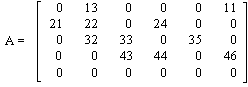
Storage by indices, also known as storage by triplets, uses three one-dimensional arrays, AR, IA, and JA, to hold the stored elements, row numbers, and column numbers respectively. Given a matrix A with ne elements to be stored, the arrays are set up as follows:
AR = ( 21, 22, 32, 33, 43, 24, 44, 35, 46, 11, 13 )
IA = ( 2, 2, 3, 3, 4, 2, 4, 3, 4, 1, 1 )
JA = ( 1, 2, 2, 3, 3, 4, 4, 5, 6, 6, 2 )
Storage by indices can be characterized as follows:
For each aij , one of the ne stored elements of the matrix A,
there exists a unique
corresponding k in [1 , ne] such that:
the kth entry of AR is aij ,
the kth entry of IA is i , and
the kth entry of JA is j .
There is an obvious one to one correspondence between the ks and the i j pairs for this storage scheme. However, determining the
k that corresponds to a particular i and j is a bit clumsy.
In short, one has to go looking for i and j to determine k.
Specifically, the k for which the kth entry of the AR array is aij is that l for which the lth entry of
IA is i and the lth entry of JA is j. This k is unique, since aij is only stored once in
AR. The following code fragment shows explicitly how to find, and change the value of, an element whose row and column indices are row_no and
col_no respectively.
  /* Inclusion of the file named "osli.h" makes possible
   *   referring to the integert control variables by name, and
   * inclusion of the file named "osli.n" makes possible
   *   referring to the index control variables by name.  */

  /* Get current values of integer and index control variables */
      ekkiget(&rtcod,dspace,osli,OSLNLI);
      ekknget(&rtcod,dspace,osln,OSLNLN);

  /* Make the initial value of k an illegal index */
   k=-1;

  /* Fine the "k" corresponding to (row_no, col_no) */
   for (j=0; j<INUMELS; j++)  {
      if (mspace[NBLOCKCOL-1 + j] == col_no &&
          mspace[NBLOCKROW-1 + j] == row_no) { k = j; break; }
   }

  /* If the value of k has become a legal index, change
   *  the value of matrix element (row_no, col_no)   */
   if (k != -1) dspace[NBLOCKELEM-1 + k] = new_value;
   else goto error;  /* element not found */
AR = ( 21, 22, 32, 13, 33, 43, 44, 24, 35, 46, 11 )
IA = ( 2, 2, 3, 1, 3, 4, 4, 2, 3, 4, 1 )
JA = ( 1, 2, 5, 7, 9, 10, 12 )
Storage by columns can be characterized as follows:
For each aij , one of the ne stored elements of the matrix A,
there exists a unique
corresponding k in [1 , ne] such that:
the kth entry of AR is aij ,
the kth entry of IA is i , and
the jth entry of JA is the l (![]() k )
for which the lth entry of AR is the first
k )
for which the lth entry of AR is the first
element, a * j , from the jth column of the
matrix A stored in AR .
( l ![]() k < l + the number of stored elements from the jth column of A ).
k < l + the number of stored elements from the jth column of A ).
For this storage scheme, there is a unique mapping from the ks to the i j pairs and vice versa. Given k , one can readily
determine i and aij . To determine j , one need only search for the first entry in the JA array that
is strictly larger k . If this entry is the lth, then j = l - 1. (Since the last entry of JA is ne + 1, there
must be such an l .) On the other hand, given i and j , we can easily find k . First obtain the value of the
jth entry of the JA array, e.g., l. Then k is the
first sequence number ![]() l for
which the corresponding entry of the IA array is i. The following code fragment shows explicitly how to find, and change the value of, an
element whose row and column indices are row_no and col_no respectively.
l for
which the corresponding entry of the IA array is i. The following code fragment shows explicitly how to find, and change the value of, an
element whose row and column indices are row_no and col_no respectively.
  /* Inclusion of the file named "osli.n" makes possible
   *   referring to the index control variables by name.  */

  /* Get current values of index control variables */
      ekknget(&rtcod,dspace,osln,OSLNLN);

  /* Make the initial value of k an illegal index */
   k=-1;

  /* Fine the "k" corresponding to (row_no, col_no) */
   for (j=mspace[NBLOCKCOL-1 + col_no-1];
        j<mspace[NBLOCKCOL-1 + col_no]; j++)   {
       if (mspace[NBLOCKROW-1 + j] == row_no) {
          k = j; break;                       }
   }

  /* If the value of k has become a legal index, change
   *  the value of matrix element (row_no, col_no)   */
   if (k != -1) dspace[NBLOCKELEM-1 + k] = new_value;
   else goto error;  /* element not found */
AR = ( 13, 11, 21, 24, 22, 32, 33, 35, 46, 44, 43 )
IA = ( 1, 3, 6, 9, 12, 12 )
JA = ( 2, 6, 1, 4, 2, 2, 3, 5, 6, 4, 3 )
In general terms, this storage technique can be expressed as follows:
For each aij , one of the ne stored elements of the matrix A,
there exists a unique
corresponding k in [1 , ne] such that:
the kth entry of AR is aij ,
the ith entry of IA is the l (![]() k) for which the lth entry
of AR is the first
k) for which the lth entry
of AR is the first
element, a i * , from the ith row of the matrix A stored in AR .
( l ![]() k < l + the number of stored elements from the ith row of A ), and
k < l + the number of stored elements from the ith row of A ), and
the kth entry of JA is j .
For this storage scheme, there is a unique mapping from the ks to the i j pairs and vice versa. Given k , one can readily
determine j and aij . To determine i , one need only search for the first entry in the IA array that
is strictly larger k . If this entry is the lth, then i = l - 1. (Since the last entry of IA is ne + 1, there
must be such an l .) On the other hand, given i and j , we can easily find k . First obtain the value of the
ith entry of the IA array, e.g., l. Then k is the first sequence number ![]() l for
which the corresponding entry of the JA array is j. We leave it as an exercise for the reader to modify the code fragment
given above (for a matrix stored by columns) to find, and change the value of, an element whose row and column indices are row_no and col_no
respectively. (Hint: interchange "NBLOCKROW" and "NBLOCKCOLUMN.")
l for
which the corresponding entry of the JA array is j. We leave it as an exercise for the reader to modify the code fragment
given above (for a matrix stored by columns) to find, and change the value of, an element whose row and column indices are row_no and col_no
respectively. (Hint: interchange "NBLOCKROW" and "NBLOCKCOLUMN.")
For some applications there may be a very large number of valid constraints. The normal way of solving these problems is to generate a model with some (often weak) constraints, solve it, see which of the larger set of constraints would tighten the problem, add these and repeat. In this case, the original matrix would be one block and the constraints (often termed cuts) could be added by EKKROW or EKKDSCB in subsequent blocks.
For most applications, only one model with one block will be needed.
If a matrix is composed of more than one block, then it may be easier to specify the size of the linear model and the bounds on the rows and columns using EKKLMDL, then pass the elements of the matrix by blocks using EKKDSCB or EKKRPTB. See "Sample FORTRAN Program EXDSCB" for an example of how to pass a model in this manner.
If you have an IBM Vector Facility, you may want to use EKKNWMT with the vector block option to improve performance. For more information, see the documentation of EKKNWMT.
You may opt to use the default values, or if you desire, you can change the value of some of the variables. This is done with the EKKxSET subroutines, where here x is one of C, I and R. (Since index control variables are not settable, there is no EKKNSET subroutine.) Some control variables are reserved for internal use. These may be examined, but not changed.
Initially, the variables are set to default values by the first library subroutine you call. The EKKINIT subroutine also resets the variables to their defaults. The default values and reference information for the control variables are provided in three places in this document:
For example, you might be solving a problem that needs to be maximized instead of the default of minimizing. In that case, you need to change the third real control variable to -1.0D0. To do this you could code in C:
      double rarray[80];
      long I80=80;
        .
        .
        .
      ekkrget(&rtcod,dspace,rarray,I80);
      rarray[2] = -1.0;
      ekkrset(&rtcod,dspace,rarray,I80);
or in FORTRAN:
      REAL*8 RARRAY(80)
        .
        .
        .
      CALL EKKRGET(RTCOD,DSPACE,RARRAY,80)
      RARRAY(3) = -1.0D0
      CALL EKKRSET(RTCOD,DSPACE,RARRAY,80)
However, you might wish to reference the control variables by mnemonic names instead of array indices. In this document, for example, all the control variables are referred to by mnemonic names. We will refer to the third real control variable as Rmaxmin, where the initial R indicates a real control variable, although you could use any name you wish.
| Note: | Throughout this document an initial R indicates a real control variable, an I indicates an integer control variable, an N indicates an index control variable, and a C indicates a character control variable. |
      REAL*8 RARRAY(80),RMAXMIN
      EQUIVALENCE (RARRAY(3),RMAXMIN)
         .
         .
         .
      CALL EKKRGET(RTCOD,DSPACE,RARRAY,80)
      RMAXMIN = -1.0D0
      CALL EKKRSET(RTCOD,DSPACE,RARRAY,80)
This method is frquently used in this document. However, it is not necessary
to enter all the required EQUIVALENCE statements and array definitions in each
sample program. All the control variable names are defined with EQUIVALENCE
statements in four INCLUDE files. The names of the C and FORTRAN include files
are:| variable type | C | FORTRAN |
| character control variables | oslc.h | OSLC |
| integer control variables | osli.h | OSLI |
| index control variables | osln.h | OSLN |
| real control variables | oslr.h | OSLR |
The following scrap of C code uses the INCLUDE files to set Rmaxmin as above, and is the form of coding used throughout this document:
      #include "oslr.h"
         .
         .
         .
      ekkrget(&rtcod,dspace,oslr,oslrln);
      RMAXMIN = -1.0;
      ekkrset(&rtcod,dspace,oslr,oslrln);
For FORTRAN programs the equivalent code would be:
      INCLUDE (OSLR)
         .
         .
         .
      CALL EKKRGET(RTCOD,DSPACE,OSLR,OSLRLN)
      RMAXMIN = -1.0D0
      CALL EKKRSET(RTCOD,DSPACE,OSLR,OSLRLN)
In this document, the ![]() symbol is used to indicate that a bit is set. For example,
symbol is used to indicate that a bit is set. For example,
1, 4 ![]() Imodelmask
indicates that the 1 and 4 bits of the integer control variable Imodelmask
are set. Imodelmask would then have a value of 9, as described above.
Imodelmask
indicates that the 1 and 4 bits of the integer control variable Imodelmask
are set. Imodelmask would then have a value of 9, as described above.
Once your subroutine has control, it could record statistics, report progress, intercept messages, change the coursed of execution, stop execution, permit execution to continue as normal, and so on. User exit routines should be coded in C or FORTRAN, and should not make any calls that could cause recursion. Refer to "Understanding User Exit Subroutines" for a more complete explanation.
dspace is a doubleword array. Sometimes, you may want to refer to information in dspace that is organized by:
   PARAMETER (NDWORDS=50000)
   DOUBLE PRECISION dspace(NDWORDS)
   INTEGER MSPACE(2*NDWORDS)
   CHARACTER*8 CSPACE(NDWORDS)
   EQUIVALENCE (dspace(1),MSPACE(1),CSPACE(1))
The row and column names can also be retrieved using EKKNAME, for details see "EKKNAME - Specify or Retrieve Names for Rows and Columns in a Model".
In some operating environments, allocating a very large dspace requires special consideration. Refer to the appropriate manuals for your particular environment.
The following is a code fragment for setting up a large 80-megabyte dspace with VS FORTRAN under an IBM host operating system:
   @PROCESS DC(BIG)
         PARAMETER (NDWORDS=10000000)
         DOUBLE PRECISION dspace(NDWORDS)
         INTEGER MSPACE(2*NDWORDS)
         CHARACTER*8 CSPACE(NDWORDS)
         COMMON/BIG/ dspace
         EQUIVALENCE (dspace(1),MSPACE(1),CSPACE(1))
A call to EKKSMAP prints out the amount of storage being used at that
moment. That is, EKKSMAP prints 1 to Nfirstfree - 1 is being used,
and Nlastfree + 1 to the size of dspace is being used.
|
|
High Storage | |
|
|
||
| Nlastfree 1
Nfirstfree 1 |
|
|
|
|
||
|
|
Low Storage |
After EKKDSCA, other subroutines may change the allocation of dspace, that is, the values of Nfirstfree and Nlastfree. Following is a description of free space, high storage, and low storage.
If you need to reserve a section of dspace for your own use, call EKKHIS as described in "High Storage".
Copies of the matrix that you make with EKKCOPY are also placed in high storage, since they are fixed in size.
Since library subroutines can change the allocation of dspace you can reserve a part of dspace for your own use with EKKHIS. This lowers Nlastfree, setting aside a section of high storage that will not be touched by library modules.
You can make storage that you have reserved with EKKHIS available for use by library modules with EKKPSHS and EKKPOPS. EKKPSHS saves the values of Nlastfree + 1 and Nfirstfree - 1. EKKPOPS restores these saved values. Therefore, if you call EKKPSHS, then EKKHIS, and finally EKKPOPS, the storage allocated by the call to EKKHIS is then "unreserved."
The subroutines that may change Nlastfree, and thus change the amount of dspace available are listed below.
The subroutines that may change Nfirstfree, and thus change the amount of dspace available are listed below.
[ Top of Page | Previous Page | Next Page | Table of Contents ]