This section describe the calling sequence arguments for vectors and matrices, and shows how to distribute vectors, matrices and sequences in a message passing program for the following areas:
An example of block-cyclic distribution of a global matrix in a Fortran 90 program in a message passing environment is shown in Appendix B. "Sample Programs". See the following:
For the Level 2 and 3 PBLAS, Dense Linear Algebraic Equations, and Eigensystem Analysis and Singular Value Analysis subroutines, certain calling sequence arguments are used to specify block-cyclically-distributed vectors or matrices.
Table 14 describes the arguments associated with a vector X. Table 15 describes the arguments associated with a matrix A.
Table 14. Calling Sequence Arguments for a Block-Cyclically-Distributed Vector
| Argument | Meaning |
|---|---|
| x | is the local part of the global matrix X. To determine the size of the local array for X, see "Determining the Number of Rows and Columns in Your Local Arrays". |
| ix | is the row index of global matrix X. |
| jx | is the column index of global matrix X. |
| desc_x | is the array descriptor for global matrix X. (See Table 16.) |
| incx | Stride for global vector X. |
| Note: | A global vector of length n is distributed across process rows the same way as an n × 1 matrix is (in this case M_X is n and N_X is 1). A global vector of length n is distributed across process columns the same way as a 1 × n matrix is (in this case M_X is 1 and N_X is n). |
Table 15. Calling Sequence Arguments for a Block-Cyclically-Distributed Matrix
| Argument | Meaning |
|---|---|
| a | is the local part of the global matrix A. To determine the size of the local array for A, see "Determining the Number of Rows and Columns in Your Local Arrays". |
| ia | is the row index of the global matrix A. |
| ja | is the column index of the global matrix A. |
| desc_a | is the array descriptor for global matrix A. (See Table 16.) |
An array descriptor, which is an integer array, is needed for each block-cyclically-distributed vector or matrix. The process grid definition and array descriptor are used to establish the mapping between the global vector or matrix and its corresponding process and distributed memory location.
Throughout this book, the _ (underscore) symbol in the array descriptor is followed by an X to indicate a vector or an A to indicate a matrix.
An example of setting up descriptor arrays in a Fortran 90 program is shown in Appendix B. "Sample Programs". See the subroutines initialize_rarray and initialize_carray in "Module Scale (Message Passing)".
Table 16 shows the type-1 array descriptor, as it is used in the Level 2 and 3 PBLAS,
Dense Linear Algebraic Equations, and Eigensystem Analysis and Singular Value
Analysis subroutines.
Table 16. Type-1 Array Descriptor for Block-Cyclically Distributed Vector or Matrix
| DESC_( ) | Symbolic name | Meaning |
|---|---|---|
| 1 | DTYPE_ | Descriptor type, where DTYPE_=1 |
| 2 | CTXT_ | BLACS context in which the global matrix is defined. (See "Initializing the BLACS".) |
| 3 | M_ | Number of rows in the global matrix |
| 4 | N_ | Number of columns in the global matrix |
| 5 | MB_ | Row block size |
| 6 | NB_ | Column block size |
| 7 | RSRC_ | The process row of the p × q process grid over which the first row of the global matrix is distributed |
| 8 | CSRC_ | The process column of the p × q process grid over which the first column of the global matrix is distributed |
| 9 | LLD_ | Leading dimension of the local array. (See "Determining the Number of Rows and Columns in Your Local Arrays".) This value may be different on each process. |
After a global vector or matrix is block-cyclically distributed over a process grid, you may decide to use only a portion of the global data structure. This is called a submatrix. For examples of how to specify the calling sequence arguments, listed in Table 14 and Table 15, for a submatrix, see:
Suppose you decide to distribute your global vector or matrix over the process grid, starting at a process other than 0,0. For examples of how to set the array descriptor values, listed in Table 16, see:
In a Parallel ESSL calling sequence, you specify an array that contains the local part of the global vector or matrix. To determine LOCp(M_) or LOCq(N_), which are used in the subroutines descriptions in Part 2 of this book, you must make a call to NUMROC:
LOCp(M_) = NUMROC (M_, MB_, myrow, RSRC_, p)
where:
LOCq(N_) = NUMROC (N_, NB_, mycol, CSRC_, q)
where:
For the Banded Linear Algebraic Equations, certain calling sequence arguments are used to specify block-cyclically distributed matrices on one-dimensional process grids.
Although the global array is block-cyclically distributed, the actual submatrix used in computation is either block-row or block-column distributed. See the appropriate subroutine for restrictions.
A symmetric band matrix must be distributed over a one-dimensional process grid:
Table 17 describes the calling sequence arguments associated with a symmetric band
matrix.
Table 17. Calling Sequence Arguments for a Distributed Symmetric Band Matrix
| Argument | Meaning |
|---|---|
| n | is the order of the global symmetric band submatrix A. |
| a | is the local part of the global symmetric band matrix A. |
| ja | is the column index of the global symmetric band matrix A. |
| desc_a | is the array descriptor for the global symmetric band matrix A. For more details, see Table 21 and Table 16. |
A general tridiagonal matrix, represented as three vectors, must be
distributed over a one-dimensional process grid using a block-cyclic data
distribution. Because vectors are one-dimensional data structures, you can use
type-501, type-502, or type-1 array descriptor regardless of whether the
process grid is p × 1 or 1 × p. Table 18 describes the calling sequence arguments associated with a general
tridiagonal matrix.
Table 18. Calling Sequence Arguments for General Tridiagonal Matrix
| Argument | Meaning |
|---|---|
| n | is the order of the global general tridiagonal submatrix A. |
| dl, d, du | is the local part of the global vectors. (The general tridiagonal matrix A is stored in tridiagonal storage mode in dl, d, and du.) |
| ia | is the row index of the global general tridiagonal matrix A. |
| desc_a | is the array descriptor for the global general tridiagonal matrix A. For more details, see Table 21, Table 16, or Table 22. |
A symmetric tridiagonal matrix, represented as two vectors, must be distributed over a one-dimensional process grid using block-cyclic data distribution.
| Note: | For both serial ESSL and Parallel ESSL, the n- 1 elements of the equal off-diagonals of a symmetric tridiagonal matrix are stored in a one-dimensional vector of length n. To be compatible with ScaLAPACK, in Parallel ESSL, the off-diagonal is chosen to be the superdiagonal and is stored in elements ia through ia+n- 2. In the serial ESSL library, the off-diagonal is chosen to be the subdiagonal and is stored in elements 2 through n. |
Because vectors are one-dimensional data structures, you can use a
type-501, type-502, or type-1 array descriptor regardless of whether the
process grid is p × 1 or 1 × p. Table 19 describes the calling sequence arguments associated with a symmetric
tridiagonal matrix.
Table 19. Calling Sequence Arguments for a Symmetric Tridiagonal Matrix
| Argument | Meaning |
|---|---|
| n | is the order of the global symmetric tridiagonal submatrix A. |
| d, e | is the local part of the global vectors. (The symmetric tridiagonal matrix A is stored in parallel-symmetric-tridiagonal storage mode in d and e.) |
| ia | is the row index of the global symmetric tridiagonal matrix A. |
| desc_a | is the array descriptor for the global symmetric tridiagonal matrix A. For more details, see Table 21, Table 16, or Table 22. |
For the Banded Linear Algebraic Equations subroutines, a general matrix consisting of multiple right-hand sides must be distributed over a one-dimensional process grid:
Table 20 describes the calling sequence arguments associated with the general matrix.
Table 20. Calling Sequence Arguments for a Matrix Containing the Multiple Right-Hand Sides
| Argument | Meaning |
|---|---|
| n | is the number of rows in the global general submatrix B. |
| b | is the local part of the global general matrix B. |
| ib | is the row index of the global general matrix B. |
| desc_b | is the array descriptor for the global general matrix B. For more details, see Table 22 and Table 16. |
An array descriptor, which is an integer array, is needed for each block-distributed matrix. The process grid definition and the array descriptor are used to establish the mapping between the global matrix and its corresponding process and distributed memory location.
In the Banded Linear Algebraic Equations sections throughout this book, the _ (underscore) symbol in the array descriptor is followed by an A or a B. A indicates a banded, tridiagonal, or symmetric tridiagonal matrix. B indicates a matrix containing the multiple right-hand sides matrix.
When you place a call to the banded or tridiagonal subroutines, you must be careful to choose consistent combinations of array descriptor types for matrix A and matrix B, and process grids. For consistent combinations, see the "Notes and Coding Rules" in the subroutine descriptions in Part 2 of this book.
Therefore, depending on which subroutine you are using in the Banded Linear Algebraic Equations, you may choose different array descriptors in the same subroutine calling sequence. Keep in mind you must only create one process grid; that is, CTXT_A = CTXT_B.
For example, when calling PDPBSV suppose you choose DTYPE_A = 501 for the
band matrix A and DTYPE_B = 502 for matrix B. If you
specify CTXT_A as 1 × p, you must also specify CTXT_B
as 1 × p. Or if you specify CTXT_A as
p × 1, you must also specify CTXT_B as
p × 1. For an example of how to set the array
descriptor values, see "Example".
Table 21. Type-501 Array Descriptor
| DESC_( ) | Symbolic name | Value |
|---|---|---|
| 1 | DTYPE_ | DTYPE_ = 501 for 1 × p or p × 1, where p is the number of processes in a process grid. |
| 2 | CTXT_ | BLACS context in which the global matrix is defined. The BLACS process
grid can be defined as 1 × p or
p × 1.
(See "Initializing the BLACS".) |
| 3 | N_ | Number of columns in the global matrix |
| 4 | NB_ | Column block size. |
| 5 | CSRC_ | The process column over which the first column of the global matrix is distributed |
| 6 | LLD_ | Leading dimension of the local array. (See "Determining the Number of Rows or Columns in Your Local Arrays".) This value may be different on each process. For the tridiagonal subroutines, this argument is ignored. |
| 7 | -- | Reserved. |
Table 22. Type-502 Array Descriptor
| DESC_( ) | Symbolic name | Value |
|---|---|---|
| 1 | DTYPE_ | DTYPE_ = 502 for p × 1 or 1 × p, where p is the number of processes in a process grid. |
| 2 | CTXT_ | BLACS context in which the global matrix is defined. The BLACS process
grid can be defined as 1 × p or
p × 1.
(See "Initializing the BLACS".) |
| 3 | M_ | Number of rows in the global matrix |
| 4 | MB_ | Row block size. |
| 5 | RSRC_ | The process row over which the first row of the global matrix is distributed |
| 6 | LLD_ | Leading dimension of the local array. (See "Determining the Number of Rows or Columns in Your Local Arrays".) This value may be different on each process. For the tridiagonal subroutines, this argument is ignored for matrix A. |
| 7 | -- | Reserved. |
For local arrays described by type-501 array descriptor, the number of rows in the local matrix is always equal to the number of rows in the global matrix. The number of columns in the local array is determined as follows:
LOCq(N_) = NUMROC(N_,NB_,mycol,CSRC_,q)
LOCq(N_) = NUMROC(N_,NB_,myrow,CSRC_,q)
where:
For local arrays described by type-502 array descriptor, the number of columns in the local matrix is always equal to the number of columns in the global matrix. The number of rows in the local array is determined as follows:
LOCp(M_) = NUMROC(M_,MB_,myrow,RSRC_,p)
LOCp(M_) = NUMROC(M_,MB_,mycol,RSRC_,p)
where:
You must distribute your data before calling Parallel ESSL from your message passing program. This section shows how you how to distribute your data.
All the Parallel ESSL message passing subroutines, except the Banded Linear Algebraic Equations and Fourier transform subroutines, support block-cyclic distribution. The Banded Linear Algebraic Equations and the Fourier transform subroutines only support block distribution.
The following sections provide examples for distributing data over one- or two-dimensional process grids:
Parallel ESSL supports block-cyclic distribution for vectors over one- or two-dimensional process grids. A vector is distributed over a single row or column of the process grid, except for PDURNG. For PDURNG, vectors are distributed block-cyclically over the entire one- or two-dimensional process grid using row-major order, where the length n of the vector x must be evenly divisible by the available processes np multiplied by the block size nb. In other words, n/(np)(nb) must be an integer.
This example shows how a global vector of length 24 with blocks of size 3 is distributed block-cyclically over one-dimensional process grids. Assume the following:
Global vector x:
B,D    0
     *    *
     | 8  |
 0   | 2  |
     | 3  |
     | -- |
     | 6  |
 1   | 5  |
     | 1  |
     | -- |
     | 9  |
 2   | 5  |
     | 3  |
     | -- |
     | 6  |
 3   | 2  |
     | 4  |
     | -- |
     | 10 |
 4   | 7  |
     | 4  |
     | -- |
     | 2  |
 5   | 8  |
     | 2  |
     | -- |
     | 8  |
 6   | 9  |
     | 2  |
     | -- |
     | 3  |
 7   | 11 |
     | 10 |
     *    *
Column-oriented, 4 × 1 process grid:
| B,D | 0 |
|---|---|
| 0
4 | P00 |
| 1
5 | P10 |
| 2
6 | P20 |
| 3
7 | P30 |
Local arrays:
p,q  | 0
-----|----
     | 8
     | 2
     | 3
 0   | 10
     | 7
     | 4
-----|----
     | 6
     | 5
     | 1
 1   | 2
     | 8
     | 2
-----|----
     | 9
     | 5
     | 3
 2   | 8
     | 9
     | 2
-----|----
     | 6
     | 2
     | 4
 3   | 3
     | 11
     | 10
For the column-oriented example, the array descriptor DESC_X
contains the following:
| DESC_X( ) | Symbolic name | Value |
|---|---|---|
| 1 | DTYPE_X | 1 |
| 2 | CTXT_X | BLACS context |
| 3 | M_X | 24 |
| 4 | N_X | 1 |
| 5 | MB_X | 3 |
| 6 | NB_X | 1 |
| 7 | RSRC_X | 0 |
| 8 | CSRC_X | 0 |
| 9 | LLD_X | 6 |
Row-oriented, 1 × 4 process grid:
| B,D | 0 4 | 1 5 | 2 6 | 3 7 |
|---|---|---|---|---|
| 0 | P00 | P01 | P02 | P03 |
Local array:
p,q  |      0        |       1       |       2       |        3
-----|---------------|---------------|---------------|----------------
 0   | 8 2 3 10 7 4  |  6 5 1 2 8 2  |  9 5 3 8 9 2  |  6 2 4 3 11 10
For the row-oriented example, the array descriptor DESC_X
contains the following:
| DESC_X( ) | Symbolic name | Value |
|---|---|---|
| 1 | DTYPE_X | 1 |
| 2 | CTXT_X | BLACS context |
| 3 | M_X | 1 |
| 4 | N_X | 24 |
| 5 | MB_X | 1 |
| 6 | NB_X | 3 |
| 7 | RSRC_X | 0 |
| 8 | CSRC_X | 0 |
| 9 | LLD_X | 1 |
| Note: | The same global vector was distributed over a 4 × 1 grid and then over a 1 × 4 grid. Notice the values contained in the corresponding local arrays are identical. |
This example shows how a global vector of length 18 with block size of 3 is distributed over two-dimensional grids. When a two-dimensional process grid is used, the global vector can be distributed over any single row or any single column of the grid. Assume the following:
Global vector x:
B,D    0
     *    *
     |  4 |
 0   | 11 |
     | 17 |
     | -- |
     | 21 |
 1   |  3 |
     |  7 |
     | -- |
     | 12 |
 2   |  5 |
     |  3 |
     | -- |
     | 15 |
 3   |  3 |
     |  4 |
     | -- |
     |  9 |
 4   | 17 |
     |  1 |
     | -- |
     | 10 |
 5   |  9 |
     | 25 |
     *    *
Two-dimensional, 2 × 3 process grid:
| B,D | -- | -- | 0 |
|---|---|---|---|
| 0
2 4 | P00 | P01 | P02 |
| 1
3 5 | P10 | P11 | P12 |
If the global vector is distributed over the third column of a 2 × 3 process grid, then P02 and P12 contain the following local arrays:
p,q  | 2
-----|----
     |  4
     | 11
     | 17
     | 12
 0   |  5
     |  3
     |  9
     | 17
     |  1
-----|----
     | 21
     |  3
     |  7
     | 15
 1   |  3
     |  4
     | 10
     |  9
     | 25
For the single column example, the array descriptor DESC_X
contains the following:
| DESC_X( ) | Symbolic name | Value |
|---|---|---|
| 1 | DTYPE_X | 1 |
| 2 | CTXT_X | BLACS context |
| 3 | M_X | 18 |
| 4 | N_X | 1 |
| 5 | MB_X | 3 |
| 6 | NB_X | 1 |
| 7 | RSRC_X | 0 |
| 8 | CSRC_X | 2 |
| 9 | LLD_X | 9 |
If the global vector is distributed over the second row of a 2 × 3 process grid, then P10, P11, and P12 contain the following local arrays:
p,q  |        0         |        1        |        2
-----|------------------|-----------------|-----------------
 1   |  4 11 17 15 3 4  |  21 3 7 9 17 1  |  12 5 3 10 9 25
For the single row example, the array descriptor DESC_X contains
the following:
| DESC_X( ) | Symbolic name | Value |
|---|---|---|
| 1 | DTYPE_X | 1 |
| 2 | CTXT_X | BLACS context |
| 3 | M_X | 1 |
| 4 | N_X | 18 |
| 5 | MB_X | 1 |
| 6 | NB_X | 3 |
| 7 | RSRC_X | 1 |
| 8 | CSRC_X | 0 |
| 9 | LLD_X | 1 |
For PDURNG, the global vector is distributed block-cyclically over the entire 2 × 3 process grid using row-major order, as follows:
p,q  |    0      |     1      |     2
-----|-----------|------------|-----------
 0   |  4 11 17  |  21  3  7  |  12  5  3
-----|-----------|------------|-----------
 1   | 15  3  4  |   9 17  1  |  10  9 25
Notes:
Following is an example of uneven block-cyclic distribution for a global vector of length 20 with block size of 3, where the two local arrays are different sizes. In this case, a fragment of a block with two elements occurs at the end of the vector. Assume the following:
X = (0, 5, 6, 3, 21, 5, 6, 1, 8, 9, 13, 11, 12, 15, 14, 15, 11, 17, 18, 19)
Following is a global vector x with block size 3:
B,D    0
     *    *
     |  0 |
 0   |  5 |
     |  6 |
     | -- |
     |  3 |
 1   | 21 |
     |  5 |
     | -- |
     |  6 |
 2   |  1 |
     |  8 |
     | -- |
     |  9 |
 3   | 13 |
     | 11 |
     | -- |
     | 12 |
 4   | 15 |
     | 14 |
     | -- |
     | 15 |
 5   | 11 |
     | 17 |
     | -- |
 6   | 18 |
     | 19 |
     *    *
Two-dimensional, 2 × 3 process grid:
| B,D | 0 | -- | -- |
|---|---|---|---|
| 0
2 4 6 | P00 | P01 | P02 |
| 1
3 5 | P10 | P11 | P12 |
If the vector is distributed over the first column of a 2 × 3 process grid, then P00 and P10 contain the following local arrays:
p,q  | 0
-----|----
     |  0
     |  5
     |  6
     |  6
     |  1
 0   |  8
     | 12
     | 15
     | 14
     | 18
     | 19
-----|----
     |  3
     | 21
     |  5
     |  9
 1   | 13
     | 11
     | 15
     | 11
     | 17
Array descriptor DESC_X contains the following:
| DESC_X( ) | Symbolic name | Value |
|---|---|---|
| 1 | DTYPE_X | 1 |
| 2 | CTXT_X | BLACS context |
| 3 | M_X | 20 |
| 4 | N_X | 1 |
| 5 | MB_X | 3 |
| 6 | NB_X | 1 |
| 7 | RSRC_X | 0 |
| 8 | CSRC_X | 0 |
| 9 | LLD_X | 11 (For P00)
9 (For P10) |
If the vector is distributed over the first row of the 2 × 3 process grid, then P00, P01, and P02 contain the following local arrays:
p,q  |           0             |         1          |         2
-----|-------------------------|--------------------|-------------------
 0   | 0  5  6  9 13 11 18 19  |  3 21  5 12 15 14  |  6  1  8 15 11 17
Array descriptor DESC_X contains the following:
| DESC_X( ) | Symbolic name | Value |
|---|---|---|
| 1 | DTYPE_X | 1 |
| 2 | CTXT_X | BLACS context |
| 3 | M_X | 1 |
| 4 | N_X | 20 |
| 5 | MB_X | 1 |
| 6 | NB_X | 3 |
| 7 | RSRC_X | 0 |
| 8 | CSRC_X | 0 |
| 9 | LLD_X | 1 |
The Parallel ESSL subroutines, except the Banded Linear Algebraic Equations, support block-cyclic data distribution for matrices using one- or two-dimensional process grids. The Banded Linear Algebraic Equations support only block data distribution using one-dimensional process grids.
The following terminology is used when it is necessary to distinguish special types of matrices:
This section describes how to distribute a matrix block-cyclically over a one-dimensional process grid. It also shows how matrices for the Banded Linear Algebraic Equations are distributed over a one-dimensional process grid using block distribution.
The examples that follow show how a 6 × 8 global matrix A with blocks of size 2 × 2 is distributed block-cyclically over one-dimensional process grids. Assume the following global matrix A:
B,D       0           1           2           3
     *                                             *
 0   |   0   1  |    2   3  |    4   5  |    6   7 |
     |  10  11  |   12  13  |   14  15  |   16  17 |
     | ---------|-----------|-----------|--------- |
 1   |  20  21  |   22  23  |   24  25  |   26  27 |
     |  30  31  |   32  33  |   34  35  |   36  37 |
     | ---------|-----------|-----------|--------- |
 2   |  40  41  |   42  43  |   44  45  |   46  47 |
     |  50  51  |   52  53  |   54  55  |   56  57 |
     *                                             *
Column-oriented, 3 × 1 process grid:
| B,D | 0 1 2 3 |
|---|---|
| 0 | P00 |
| 1 | P10 |
| 2 | P20 |
Local arrays:
p,q  |                0
-----|---------------------------------
 0   |   0   1   2   3   4   5   6   7
     |  10  11  12  13  14  15  16  17
-----|---------------------------------
 1   |  20  21  22  23  24  25  26  27
     |  30  31  32  33  34  35  36  37
-----|---------------------------------
 2   |  40  41  42  43  44  45  46  47
     |  50  51  52  53  54  55  56  57
For the column-oriented example, the array descriptor DESC_A
contains:
| DESC_A( ) | Symbolic name | Value |
|---|---|---|
| 1 | DTYPE_A | 1 |
| 2 | CTXT_A | BLACS context |
| 3 | M_A | 6 |
| 4 | N_A | 8 |
| 5 | MB_A | 2 |
| 6 | NB_A | 2 |
| 7 | RSRC_A | 0 |
| 8 | CSRC_A | 0 |
| 9 | LLD_A | 2 |
Row-oriented, 1 × 2 process grid:
| B,D | 0 2 | 1 3 |
|---|---|---|
| 0
1 2 | P00 | P01 |
Local arrays:
p,q  |        0         |         1
-----|------------------|------------------
     |   0   1   4   5  |    2   3   6   7
     |  10  11  14  15  |   12  13  16  17
     |  20  21  24  25  |   22  23  26  27
 0   |  30  31  34  35  |   32  33  36  37
     |  40  41  44  45  |   42  43  46  47
     |  50  51  54  55  |   52  53  56  57
For the row-oriented example, the array descriptor DESC_A:
| DESC_A( ) | Symbolic name | Value |
|---|---|---|
| 1 | DTYPE_A | 1 |
| 2 | CTXT_A | BLACS context |
| 3 | M_A | 6 |
| 4 | N_A | 8 |
| 5 | MB_A | 2 |
| 6 | NB_A | 2 |
| 7 | RSRC_A | 0 |
| 8 | CSRC_A | 0 |
| 9 | LLD_A | 6 |
For an example of distributing a matrix over a one-dimensional process grid in a Fortran 90 program, see matrix F in Appendix B. "Sample Programs", which is:
This section shows how to distribute a symmetric band matrix A over a one-dimensional process grid using block-cyclic distribution.
Assume the following symmetric band matrix A of size 9 × 9 with a half bandwidth of 2:
              *                                  *
              | 11  21  31   0   0   0   0  0  0 |
              | 21  22  32  42   0   0   0  0  0 |
              | 31  32  33  34  53   0   0  0  0 |
         A =  |  0  42  34  44  54  64   0  0  0 |
              |  0   0  53  54  55  65  75  0  0 |
              |  0   0   0  64  65  66  76 86  0 |
              |  0   0   0   0  75  76  77 87 97 |
              |  0   0   0   0   0  86  87 88 98 |
              |  0   0   0   0   0   0  97 98 99 |
              *                                  *
Matrix A must be stored in upper- or lower-band-packed storage mode. The sections that follow contain examples describing these two storage modes. In these examples, matrix A is stored in an array with dimensions 3 × 9.
The global matrix A with block size of 2 is stored in upper-band-packed storage mode, as follows:
B,D      0       1       2       3      4
     *                                    *
     |  *  * | 31 42 | 53 64 | 75 86 | 97 |
 0   |  * 21 | 32 34 | 54 65 | 76 87 | 98 |
     | 11 22 | 33 44 | 55 66 | 77 88 | 99 |
     *                                    *
Following is a row-oriented, 1 × 3 process grid:
| B,D | 0 3 | 1 4 | 2 |
|---|---|---|---|
| 0 | P00 | P01 | P02 |
The following local arrays A are distributed block-cyclically over the 1 × 3 process grid:
p,q  |      0       |     1     |    2
-----|--------------|-----------|--------
     |  *  *  75 86 |  31 42 97 |  53 64
 0   |  * 21  76 87 |  32 34 98 |  54 65
     | 11 22  77 88 |  33 44 99 |  55 66
where * means you do not have to store a value in that position in the local array. However, these storage positions are required and overwritten during the computation.
The type-501 array descriptor DESC_A contains the
following:
| DESC_A( ) | Symbolic name | Value |
|---|---|---|
| 1 | DTYPE_A | DTYPE_A = 501 for 1 × p |
| 2 | CTXT_A | BLACS context |
| 3 | N_A | 9 |
| 4 | NB_A | 2 |
| 5 | CSRC_A | 0 |
| 6 | LLD_A | 3 |
| 7 | -- | Reserved |
Alternately, the type-1 array descriptor DESC_A contains the
following:
| DESC_A( ) | Symbolic name | Value |
|---|---|---|
| 1 | DTYPE_A | DTYPE_A = 1 for 1 × p |
| 2 | CTXT_A | BLACS context |
| 3 | M_A | 3 |
| 4 | N_A | 9 |
| 5 | MB_A | 1 |
| 6 | NB_A | 2 |
| 7 | RSRC_A | 0 |
| 8 | CSRC_A | 0 |
| 9 | LLD_A | 3 |
The global matrix A with block size of 2 is stored in lower-band-packed storage mode, as follows:
B,D      0       1       2       3      4
     *                                    *
     | 11 22 | 33 44 | 55 66 | 77 88 | 99 |
 0   | 21 32 | 34 54 | 65 76 | 87 98 |  * |
     | 31 42 | 53 64 | 75 86 | 97  * |  * |
     *                                    *
Following is a row-oriented, 1 × 3 process grid:
| B,D | 0 3 | 1 4 | 2 |
|---|---|---|---|
| 0 | P00 | P01 | P02 |
The following local arrays A are distributed block-cyclically over the 1 × 3 process grid:
p,q  |      0      |     1    |    2
-----|-------------|----------|--------
     | 11 22 77 88 | 33 44 99 | 55 66
 0   | 21 32 87 98 | 34 54  * | 65 76
     | 31 42 97  * | 53 64  * | 75 86
where * means you do not have to store a value in that position in the local array. However, these storage positions are required and overwritten during the computation.
The type-501 array descriptor DESC_A contains the
following:
| DESC_A( ) | Symbolic name | Value |
|---|---|---|
| 1 | DTYPE_A | DTYPE_A = 501 for 1 × p |
| 2 | CTXT_A | BLACS context |
| 3 | N_A | 9 |
| 4 | NB_A | 2 |
| 5 | CSRC_A | 0 |
| 6 | LLD_A | 3 |
| 7 | -- | Reserved |
Alternately, the type-1 array descriptor DESC_A contains the
following:
| DESC_A( ) | Symbolic name | Value |
|---|---|---|
| 1 | DTYPE_A | DTYPE_A = 1 for 1 × p |
| 2 | CTXT_A | BLACS context |
| 3 | M_A | 3 |
| 4 | N_A | 9 |
| 5 | MB_A | 1 |
| 6 | NB_A | 2 |
| 7 | RSRC_A | 0 |
| 8 | CSRC_A | 0 |
| 9 | LLD_A | 3 |
For more information on how to store symmetric band matrices, see the ESSL Version 3 Guide and Reference manual.
A general tridiagonal matrix, represented as three vectors, must be distributed over a one-dimensional process grid using a block-cyclic data distribution. Because vectors are one-dimensional data structures, you can use a type-501, type-502, or type-1 array descriptor regardless of whether the process grid is 1 × p or p × 1.
The first part of this section shows how to distribute a general tridiagonal matrix A over a p × 1 process grid. The second part shows how to distribute the same matrix over a 1 × p process grid. In both cases, the values contained in the corresponding local arrays are identical.
Assume the following general tridiagonal matrix A of size 7 × 7:
              *                          *
              | 11  12   0   0   0  0  0 |
              | 21  22  23   0   0  0  0 |
              |  0  32  33  34   0  0  0 |
              |  0   0  43  44  45  0  0 |
              |  0   0   0  54  55 56  0 |
              |  0   0   0   0  65 66 67 |
              |  0   0   0   0   0 76 77 |
              *                          *
Matrix A is stored in tridiagonal storage mode in the following three vectors:
dl= (*, 21, 32, 43, 54, 65, 76)
d= (11, 22, 33, 44, 55, 66, 77)
du= (12, 23, 34, 45, 56, 67, *)
The general tridiagonal matrix A is stored in tridiagonal storage mode in vectors dl, d, and du.
Following is global vector dl:
B,D    0
     *    *
 0   |  * |
     | 21 |
     | -- |
 1   | 32 |
     | 43 |
     | -- |
 2   | 54 |
     | 65 |
     | -- |
 3   | 76 |
     *    *
Following is global vector d:
B,D    0
     *    *
 0   | 11 |
     | 22 |
     | -- |
 1   | 33 |
     | 44 |
     | -- |
 2   | 55 |
     | 66 |
     | -- |
 3   | 77 |
     *    *
Following is global vector du:
B,D    0
     *    *
 0   | 12 |
     | 23 |
     | -- |
 1   | 34 |
     | 45 |
     | -- |
 2   | 56 |
     | 67 |
     | -- |
 3   |  * |
     *    *
Following is a column-oriented, 3 × 1 process grid:
| B,D | 0 |
|---|---|
| 0
3 | P00 |
| 1 | P10 |
| 2 | P20 |
The arrays are block-cyclically distributed over the 3 × 1 process grid.
Following are the local arrays for DL:
p,q  | 0
-----|----
 0   |  *
     | 21
     | 76
-----|----
 1   | 32
     | 43
-----|----
 2   | 54
     | 65
Following are the local arrays for D:
p,q  | 0
-----|----
 0   | 11
     | 22
     | 77
-----|----
 1   | 33
     | 44
-----|----
 2   | 55
     | 66
Following are the local arrays for DU:
p,q  | 0
-----|----
 0   | 12
     | 23
     |  *
-----|----
 1   | 34
     | 45
-----|----
 2   | 56
     | 67
where "*" means you do not have to store a value in that position in the local array. However, these storage positions are required.
The type-502 array descriptor DESC_A contains the
following:
| DESC_A( ) | Symbolic name | Value |
|---|---|---|
| 1 | DTYPE_A | DTYPE_A = 502 for p × 1 |
| 2 | CTXT_A | BLACS context |
| 3 | M_A | 7 |
| 4 | MB_A | 2 |
| 5 | RSRC_A | 0 |
| 6 | LLD_A | Not used |
| 7 | - | Reserved |
Alternately, the type-1 array descriptor DESC_A contains the
following:
| DESC_A( ) | Symbolic name | Value |
|---|---|---|
| 1 | DTYPE_A | DTYPE_A = 1 for p × 1 |
| 2 | CTXT_A | BLACS context |
| 3 | M_A | 7 |
| 4 | N_A | 1 |
| 5 | MB_A | 2 |
| 6 | NB_A | 1 |
| 7 | RSRC_A | 0 |
| 8 | CSRC_A | 0 |
| 9 | LLD_A | Not used |
The general tridiagonal matrix A is stored in tridiagonal storage mode in vectors dl, d, and du. Because vectors are one-dimensional data structures, the block-cyclically distributed arrays on a 1 × p process grid are identical to the block-cyclically distributed arrays on a p × 1 process grid.
Following is global vector dl:
B,D     0       1       2      3
     *                           *
 0   | * 21 | 32 43 | 54 65 | 76 |
     *                           *
Following is global vector d:
B,D      0       1       2      3
     *                            *
 0   | 11 22 | 33 44 | 55 66 | 77 |
     *                            *
Following is global vectors du:
B,D      0       1       2      3
     *                             *
 0   | 12 23 | 34 45 | 55 67 |  *  |
     *                             *
Following is a row-oriented, 1 × 3 process grid:
| B,D | 0 3 | 1 | 2 |
|---|---|---|---|
| 0 | P00 | P01 | P02 |
The arrays are block-cyclically distributed over the 1 × 3 process grid.
Following are the local arrays for DL:
p,q  |     0   |   1   |   2
-----|---------|-------|------
 0   | * 21 76 | 32 43 | 54 65
Following are the local arrays for D:
p,q  |     0    |   1   |   2
-----|----------|-------|------
 0   | 11 22 77 | 33 44 | 55 66
Following are the local arrays for DU:
p,q  |   0      |    1   |   2
-----|----------|--------|-------
 0   | 12 23  * | 34 45  | 55 67
where "*" means you do not have to store a value in that position in the local array. However, these storage positions are required.
The type-501 array descriptor DESC_A contains the
following:
| DESC_A( ) | Symbolic name | Value |
|---|---|---|
| 1 | DTYPE_A | DTYPE_A = 501 for 1 × p |
| 2 | CTXT_A | BLACS context |
| 3 | N_A | 7 |
| 4 | NB_A | 2 |
| 5 | CSRC_A | 0 |
| 6 | LLD_A | Not used |
| 7 | - | Reserved |
Alternately, the type-1 array descriptor DESC_A contains the
following:
| DESC_A( ) | Symbolic name | Value |
|---|---|---|
| 1 | DTYPE_A | DTYPE_A = 1 for 1 × p |
| 2 | CTXT_A | BLACS context |
| 3 | M_A | 1 |
| 4 | N_A | 7 |
| 5 | MB_A | 1 |
| 6 | NB_A | 2 |
| 7 | RSRC_A | 0 |
| 8 | CSRC_A | 0 |
| 9 | LLD_A | Not used |
For more information on how to store general tridiagonal matrices, see the ESSL Version 3 Guide and Reference manual.
A symmetric tridiagonal matrix, represented as two vectors, must be distributed over a one-dimensional process grid using a block-cyclic data distribution. Because vectors are one-dimensional data structures, you can use a type-501, type-502, or type-1 array descriptor regardless of whether the process grid is p × 1 or 1 × p.
| Note: | For both serial ESSL and Parallel ESSL, the n- 1 elements of the equal off-diagonals of a symmetric tridiagonal matrix are stored in a one-dimensional vector of length n. To be compatible with ScaLAPACK, in Parallel ESSL, the off-diagonal is chosen to be the superdiagonal and is stored in elements 1 through n- 1. In the serial ESSL library, the off-diagonal is chosen to be the subdiagonal and is stored in elements 2 through n. |
The first part of this section shows a how to distribute a symmetric tridiagonal matrix A over a p × 1 process grid. The second part shows how to distribute the same matrix over a 1 × p process grid. In both cases, the values contained in the corresponding local arrays are identical.
Assume the following symmetric tridiagonal matrix A of size 7 × 7:
              *                           *
              | 10   1   0   0   0   0  0 |
              |  1  20   2   0   0   0  0 |
              |  0   2  30   3   0   0  0 |
              |  0   0   3  40   4   0  0 |
              |  0   0   0   4  50   5  0 |
              |  0   0   0   0   5  60  6 |
              |  0   0   0   0   0   6 70 |
              *                           *
Matrix A is stored in parallel-symmetric-tridiagonal storage mode in the following two vectors:
d= (10, 20, 30, 40, 50, 60, 70)
e= (1, 2, 3, 4, 5, 6, *)
The symmetric tridiagonal matrix A is stored in parallel-symmetric-tridiagonal storage mode in vectors d and e.
Following is global vector d:
B,D    0
     *    *
     | 10 |
 0   | 20 |
     | 30 |
     | -- |
 1   | 40 |
     | 50 |
     | 60 |
     | -- |
 2   | 70 |
     *    *
Following is global vector e:
B,D    0
     *   *
     | 1 |
 0   | 2 |
     | 3 |
     | - |
 1   | 4 |
     | 5 |
     | 6 |
     | - |
 2   | * |
     *   *
Following is a column-oriented, 2 × 1 process grid:
| B,D | 0 |
|---|---|
| 0
2 | P00 |
| 1 | P10 |
The arrays are block-cyclically distributed over the 2 × 1 process grid.
Following are the local arrays for D:
p,q  | 0
-----|----
     | 10
 0   | 20
     | 30
     | 70
-----|----
 1   | 40
     | 50
     | 60
Following are the local arrays for E:
p,q  | 0
-----|---
     | 1
 0   | 2
     | 3
     | *
-----|---
 1   | 4
     | 5
     | 6
where * means you do not have to store a value in that position in the local array. However, these storage positions are required.
The type-502 array descriptor DESC_A contains the
following:
| DESC_A( ) | Symbolic name | Value |
|---|---|---|
| 1 | DTYPE_A | DTYPE_A = 502 for p × 1 |
| 2 | CTXT_A | BLACS context |
| 3 | M_A | 7 |
| 4 | MB_A | 3 |
| 5 | RSRC_A | 0 |
| 6 | LLD_A | Not used |
| 7 | - | Reserved |
Alternately, the type-1 array descriptor DESC_A contains the
following:
| DESC_A( ) | Symbolic name | Value |
|---|---|---|
| 1 | DTYPE_A | DTYPE_A = 1 for p × 1 |
| 2 | CTXT_A | BLACS context |
| 3 | M_A | 7 |
| 4 | N_A | 1 |
| 5 | MB_A | 3 |
| 6 | NB_A | 1 |
| 7 | RSRC_A | 0 |
| 8 | CSRC_A | 0 |
| 9 | LLD_A | Not used |
The symmetric tridiagonal matrix A is stored in parallel-symmetric-tridiagonal storage mode in vectors d and e. Because vectors are one-dimensional data structures, the block-cyclically distributed arrays on a 1 × p process grid are identical to the block-cyclically distributed arrays on a p × 1 process grid.
Following is global vector d:
B,D        0          1       2
     *                          *
 0   | 10 20 30 | 40 50 60 | 70 |
     *                          *
Following is global vector e:
B,D      0       1     2
     *                   *
 0   | 1 2 3 | 4 5 6 | * |
     *                   *
Following is a row-oriented, 1 × 2 process grid:
| B,D | 0 2 | 1 |
|---|---|---|
| 0 | P00 | P01 |
The arrays are block-cyclically distributed over the 1 × 2 process grid.
Following are the local arrays for D:
p,q  |      0       |    1
-----|--------------|---------
 0   | 10 20 30 70  | 40 50 60
Following are the local arrays for E:
p,q  |    0    |   1
-----|---------|------
 0   | 1 2 3 * | 4 5 6
where "*" means you do not have to store a value in that position in the local array. However, these storage positions are required.
The type-501 array descriptor DESC_A contains the
following:
| DESC_A( ) | Symbolic name | Value |
|---|---|---|
| 1 | DTYPE_A | DTYPE_A = 501 for 1 × p |
| 2 | CTXT_A | BLACS context |
| 3 | N_A | 7 |
| 4 | NB_A | 3 |
| 5 | CSRC_A | 0 |
| 6 | LLD_A | Not used |
| 7 | - | Reserved |
Alternately, the type-1 array descriptor DESC_A contains the
following:
| DESC_A( ) | Symbolic name | Value |
|---|---|---|
| 1 | DTYPE_A | DTYPE_A = 1 for 1 × p |
| 2 | CTXT_A | BLACS context |
| 3 | M_A | 1 |
| 4 | N_A | 7 |
| 5 | MB_A | 1 |
| 6 | NB_A | 3 |
| 7 | RSRC_A | 0 |
| 8 | CSRC_A | 0 |
| 9 | LLD_A | Not used |
This section shows how to block-cyclically distribute a general matrix B containing the multiple right-hand sides for the Banded Linear Algebraic Equations subroutines.
Following is the global matrix B:
B,D       0
     *          *
 0   | 11 12 13 |
     | 21 22 23 |
     | -------- |
 1   | 31 32 33 |
     | 41 42 43 |
     | -------- |
 2   | 51 52 53 |
     | 61 62 63 |
     |----------|
 3   | 71 72 73 |
     *          *
Following is a 3 × 1 process grid:
| B,D | 0 |
|---|---|
| 0
3 | P00 |
| 1 | P10 |
| 2 | P20 |
Following are the local arrays:
p,q  |    0
-----|----------
 0   | 11 12 13
     | 21 22 23
     | 71 72 73
-----|----------
 1   | 31 32 33
     | 41 42 43
-----|----------
 2   | 51 52 53
     | 61 62 63
The type-502 array descriptor DESC_B contains the
following:
| DESC_B( ) | Symbolic name | Value |
|---|---|---|
| 1 | DTYPE_B | DTYPE_B = 502 for p × 1 |
| 2 | CTXT_B | BLACS context |
| 3 | M_B | 7 |
| 4 | MB_B | 2 |
| 5 | RSRC_B | 0 |
| 6 | LLD_B | 3 (For P00)
2 (For P10 and P20) |
| 7 | -- | Reserved |
Alternately, the type-1 array descriptor DESC_B contains the
following:
| DESC_B( ) | Symbolic name | Value |
|---|---|---|
| 1 | DTYPE_B | DTYPE_B = 1 for p × 1 |
| 2 | CTXT_B | BLACS context |
| 3 | M_B | 7 |
| 4 | N_B | 3 |
| 5 | MB_B | 2 |
| 6 | NB_B | 1 |
| 7 | RSRC_B | 0 |
| 8 | CSRC_B | 0 |
| 9 | LLD_B | 3 (For P00)
2 (For P10 and P20) |
This section shows how to distribute general, symmetric, and upper triangular matrices over a two-dimensional process grid using block-cyclic distribution.
This example shows how the data for a global matrix A with block size of 2 × 3 is distributed block-cyclically over the entire 2 × 3 process grid. Assume the following 9 × 26 global matrix A with 45 blocks:
B,D       0          1         2         3          4           5         6          7         8
     *                                                                                            *
 0   | 112 5 7  |  8 9 3  |  7 5 1  |  3 2 1  |  8 98   4  |  8 9 4  |  1 3 10  |  3 3 10  |  5 3 |
     | 116 9 6  |  7 2 3  |  6 5 6  |  4 3 2  |  7  2 111  |  7 2 1  |  7 6 15  |  7 6 15  |  7 6 |
     | ---------|---------|---------|---------|------------|---------|----------|----------|----- |
 1   |   1 5 7  |  1 9 3  |  1 5 1  |  1 2 1  |  1  9   4  |  1 9 4  |  5 8 10  |  3 3 11  |  5 3 |
     |   6 9 6  |  7 2 3  |  6 5 6  |  4 3 2  |  7  2   1  |  7 2 1  |  7 6 19  |  7 1 15  |  7 2 |
     | ---------|---------|---------|---------|------------|---------|----------|----------|----- |
 2   |   2 5 7  |  2 9 3  |  2 5 1  |  2 2 1  |  2  9   4  |  2 9 4  |  1 8 10  |  2 3 11  |  3 3 |
     |   6 9 6  |  7 2 3  |  6 5 6  |  4 3 2  |  7  2   1  |  7 2 1  |  7 3 19  |  7 4 15  |  7 8 |
     | ---------|---------|---------|---------|------------|---------|----------|----------|----- |
 3   |   3 5 7  |  3 9 3  |  3 5 1  |  3 2 1  |  3  9   4  |  3 9 4  |  9 8 10  |  2 3 11  |  3 3 |
     |   6 9 6  |  7 2 3  |  6 5 6  |  4 3 2  |  7  2   1  |  7 2 1  |  1 3 49  |  7 4 55  |  7 3 |
     | ---------|---------|---------|---------|------------|---------|----------|----------|----- |
 4   |  20 1 9  |  4 5 6  |  9 8 7  |  1 4 3  |  1 15  21  |  4 7 6  |  9 8 12  |  3 9 18  |  2 4 |
     *                                                                                            *
| Note: | In this example, the global matrix dimensions are not divisible by the respective block size. As a result, all of the block sizes are 2 × 3, except for blocks in the last row and the last column of the blocked matrix. |
Two-dimensional, 2 × 3 process grid:
| B,D | 0 3 6 | 1 4 7 | 2 5 8 |
|---|---|---|---|
| 0
2 4 | P00 | P01 | P02 |
| 1
3 | P10 | P11 | P12 |
Local arrays:
p,q  |          0            |            1            |         2
-----|-----------------------|-------------------------|------------------
     | 112 5 7 3 2 1 1 3 10  |  8 9 3 8 98   4 3 3 10  |  7 5 1 8 9 4 5 3
     | 116 9 6 4 3 2 7 6 15  |  7 2 3 7  2 111 7 6 15  |  6 5 6 7 2 1 7 6
 0   |   2 5 7 2 2 1 1 8 10  |  2 9 3 2  9   4 2 3 11  |  2 5 1 2 9 4 3 3
     |   6 9 6 4 3 2 7 3 19  |  7 2 3 7  2   1 7 4 15  |  6 5 6 7 2 1 7 8
     |  20 1 9 1 4 3 9 8 12  |  4 5 6 1 15  21 3 9 18  |  9 8 7 4 7 6 2 4
-----|-----------------------|-------------------------|------------------
     |   1 5 7 1 2 1 5 8 10  |  1 9 3 1  9   4 3 3 11  |  1 5 1 1 9 4 5 3
     |   6 9 6 4 3 2 7 6 19  |  7 2 3 7  2   1 7 1 15  |  6 5 6 7 2 1 7 2
 1   |   3 5 7 3 2 1 9 8 10  |  3 9 3 3  9   4 2 3 11  |  3 5 1 3 9 4 3 3
     |   6 9 6 4 3 2 1 3 49  |  7 2 3 7  2   1 7 4 55  |  6 5 6 7 2 1 7 3
Array descriptor DESC_A contains the following:
| DESC_A( ) | Symbolic name | Value |
|---|---|---|
| 1 | DTYPE_A | 1 |
| 2 | CTXT_A | BLACS context |
| 3 | M_A | 9 |
| 4 | N_A | 26 |
| 5 | MB_A | 2 |
| 6 | NB_A | 3 |
| 7 | RSRC_A | 0 |
| 8 | CSRC_A | 0 |
| 9 | LLD_A | 5 (For P00, P01, and P02)
4 (For P10, P11, and P12) |
This example shows how the data for a global symmetric matrix A with block size of 3 × 3 is distributed block-cyclically over a 2 × 3 process grid. Assume the following 18 × 18 global symmetric matrix A with 36 blocks:
B,D       0            1            2            3            4            5
     *                                                                           *
     |  1  2  3  |   4  5  6  |   7  8  9  |  10 11 12  |  13 14 15  |  16 17 18 |
 0   |  2 10 11  |  12 13 14  |  15 16 17  |  18 19 20  |  21 22 23  |  24 25 26 |
     |  3 11 20  |  21 22 23  |  24 25 26  |  27 28 29  |  30 31 32  |  33 34 35 |
     | ----------|------------|------------|------------|------------|---------- |
     |  4 12 21  |   2  3  5  |   7 11 13  |  17 19 23  |  29 31 37  |  41 43 47 |
 1   |  5 13 22  |   3  1  4  |   9 16 25  |  36 49 64  |  81 10 12  |  14 16 19 |
     |  6 14 23  |   5  4  5  |   6 10 11  |  15 16 20  |  21 25 26  |  30 31 35 |
     | ----------|------------|------------|------------|------------|---------- |
     |  7 15 24  |   7  9  6  |   1  2  3  |   4  5  6  |   7  8  9  |  10 11 12 |
 2   |  8 16 25  |  11 16 10  |   2 11 13  |  15 17 19  |  21 23 25  |  27 29 31 |
     |  9 17 26  |  13 25 11  |   3 13  2  |   4  6  8  |  10 12 14  |  16 18 20 |
     | ----------|------------|------------|------------|------------|---------- |
     | 10 18 27  |  17 36 15  |   4 15 4   |   3  6  9  |   2  4  6  |   3  6  9 |
 3   | 11 19 28  |  19 49 16  |   5 17 6   |   6  1  2  |   3  4  5  |   6  7  8 |
     | 12 20 29  |  23 64 20  |   6 19 8   |   9  2  1  |   3  5  7  |   9 11 13 |
     | ----------|------------|------------|------------|------------|---------- |
     | 13 21 30  |  29 81 21  |   7 21 10  |   2  3  3  |  20 22 21  |  24 23 25 |
 4   | 14 22 31  |  31 10 25  |   8 23 12  |   4  4  5  |  22  4  5  |   6  9 10 |
     | 15 23 32  |  37 12 26  |   9 25 14  |   6  5  7  |  21  5  3  |   2  7  8 |
     | ----------|------------|------------|------------|------------|---------- |
     | 16 24 33  |  41 14 30  |  10 27 16  |   3  6  9  |  24  6  2  |   4 11 15 |
 5   | 17 25 34  |  43 16 31  |  11 29 18  |   6  7 11  |  23  9  7  |  11 17 13 |
     | 18 26 35  |  47 19 35  |  12 31 20  |   9  8 13  |  25 10  8  |  15 13 21 |
     *                                                                           *
Two-dimensional, 3 × 2 process grid:
| B,D | 0 2 4 | 1 3 5 |
|---|---|---|
| 0
3 | P00 | P01 |
| 1
4 | P10 | P11 |
| 2
5 | P20 | P21 |
The symmetric matrix is distributed block-cyclically in lower storage mode over a 3 × 2 process grid:
p,q  |             0               |              1
-----|-----------------------------|-----------------------------
     |  1  *  *  *  *  *  *  *  *  |   *  *  *  *  *  *  *  *  *
     |  2 10  *  *  *  *  *  *  *  |   *  *  *  *  *  *  *  *  *
     |  3 11 20  *  *  *  *  *  *  |   *  *  *  *  *  *  *  *  *
 0   | 10 18 27  4 15  4  *  *  *  |  17 36 15  3  *  *  *  *  *
     | 11 19 28  5 17  6  *  *  *  |  19 49 16  6  1  *  *  *  *
     | 12 20 29  6 19  8  *  *  *  |  23 64 20  9  2  1  *  *  *
-----|-----------------------------|-----------------------------
     |  4 12 21  *  *  *  *  *  *  |   2  *  *  *  *  *  *  *  *
     |  5 13 22  *  *  *  *  *  *  |   3  1  *  *  *  *  *  *  *
     |  6 14 23  *  *  *  *  *  *  |   5  4  5  *  *  *  *  *  *
 1   | 13 21 30  7 21 10 20  *  *  |  29 81 21  2  3  3  *  *  *
     | 14 22 31  8 23 12 22  4  *  |  31 10 25  4  4  5  *  *  *
     | 15 23 32  9 25 14 21  5  3  |  37 12 26  6  5  7  *  *  *
-----|-----------------------------|-----------------------------
     |  7 15 24  1  *  *  *  *  *  |   7  9  6  *  *  *  *  *  *
     |  8 16 25  2 11  *  *  *  *  |  11 16 10  *  *  *  *  *  *
     |  9 17 26  3 13  2  *  *  *  |  13 25 11  *  *  *  *  *  *
 2   | 16 24 33 10 27 16 24  6  2  |  41 14 30  3  6  9  4  *  *
     | 17 25 34 11 29 18 23  9  7  |  43 16 31  6  7 11 11 17  *
     | 18 26 35 12 31 20 25 10  8  |  47 19 35  9  8 13 15 13 21
where * means you do not have to store a value in that position in the local array. However, these storage positions are required.
Notice that the local arrays are not symmetric.
Array descriptor DESC_A contains the following:
| DESC_A( ) | Symbolic name | Value |
|---|---|---|
| 1 | DTYPE_A | 1 |
| 2 | CTXT_A | BLACS context |
| 3 | M_A | 18 |
| 4 | N_A | 18 |
| 5 | MB_A | 3 |
| 6 | NB_A | 3 |
| 7 | RSRC_A | 0 |
| 8 | CSRC_A | 0 |
| 9 | LLD_A | 6 |
For more information on how to store symmetric matrices, see the ESSL Version 3 Guide and Reference manual.
This example shows how the data for a global upper triangular matrix A with block size of 2 × 2 is distributed block-cyclically over a 2 × 3 process grid. Assume the following 12 × 12 global upper triangular matrix A with 36 blocks:
B,D      0         1         2         3         4         5
     *                                                         *
 0   |  2  1  |   2 13  |  13 10  |  15 21  |  26 31  |   7  5 |
     |  0  3  |   4  4  |  11 23  |  41 45  |  59 67  |   1  8 |
     | -------|---------|---------|---------|---------|------- |
 1   |  0  0  |   5  9  |   6  9  |  33 65  |  21 14  |   9  4 |
     |  0  0  |   0  7  |  16  8  |   7 33  |   3  7  |   5  3 |
     | -------|---------|---------|---------|---------|------- |
 2   |  0  0  |   0  0  |  11 25  |  10  5  |  23  7  |  10  6 |
     |  0  0  |   0  0  |   0 13  |  36 12  |   3 13  |   5  6 |
     | -------|---------|---------|---------|---------|------- |
 3   |  0  0  |   0  0  |   0  0  |  17 49  |  14  1  |   7  2 |
     |  0  0  |   0  0  |   0  0  |   0 19  |  64 16  |   1  7 |
     | -------|---------|---------|---------|---------|------- |
 4   |  0  0  |   0  0  |   0  0  |   0  0  |  23 81  |   6 15 |
     |  0  0  |   0  0  |   0  0  |   0  0  |   0 29  |   9  4 |
     | -------|---------|---------|---------|---------|------- |
 5   |  0  0  |   0  0  |   0  0  |   0  0  |   0  0  |   5  3 |
     |  0  0  |   0  0  |   0  0  |   0  0  |   0  0  |   0  4 |
     *                                                         *
Two-dimensional, 2 × 3 process grid:
| B,D | 0 3 | 1 4 | 2 5 |
|---|---|---|---|
| 0
2 4 | P00 | P01 | P02 |
| 1
3 5 | P10 | P11 | P12 |
The following local arrays are distributed block-cyclically in upper-triangular storage mode over a 2 × 3 process grid:
p,q  |      0       |       1       |       2
-----|--------------|---------------|--------------
     |  2  1 15 21  |   2 13 26 31  |  13 10  7  5
     |  *  3 41 45  |   4  4 59 67  |  11 23  1  8
     |  *  * 10  5  |   *  * 23  7  |  11 25 10  6
 0   |  *  * 36 12  |   *  *  3 13  |   * 13  5  6
     |  *  *  *  *  |   *  * 23 81  |   *  *  6 15
     |  *  *  *  *  |   *  *  * 29  |   *  *  9  4
-----|--------------|---------------|--------------
     |  *  * 33 65  |   5  9 21 14  |   6  9  9  4
     |  *  *  7 33  |   *  7  3  7  |  16  8  5  3
     |  *  * 17 49  |   *  * 14  1  |   *  *  7  2
 1   |  *  *  * 19  |   *  * 64 16  |   *  *  1  7
     |  *  *  *  *  |   *  *  *  *  |   *  *  5  3
     |  *  *  *  *  |   *  *  *  *  |   *  *  *  4
where "*" means you do not have to store a value in that position in the local array. However, these storage positions are required.
Notice the local arrays are not upper triangular.
Array descriptor DESC_A contains the following:
| DESC_A( ) | Symbolic name | Value |
|---|---|---|
| 1 | DTYPE_A | 1 |
| 2 | CTXT_A | BLACS context |
| 3 | M_A | 12 |
| 4 | N_A | 12 |
| 5 | MB_A | 2 |
| 6 | NB_A | 2 |
| 7 | RSRC_A | 0 |
| 8 | CSRC_A | 0 |
| 9 | LLD_A | 6 |
For more information on how to store triangular matrices, see the ESSL Version 3 Guide and Reference manual.
For the Fortran 90 and Fortran 77 sparse linear algebraic equation subroutines, you must use the sparse utility subroutines provided with Parallel ESSL to build the sparse matrices on each process in the process grid. This sections shows the calling sequence arguments associated with the sparse matrix A.
This section contains the following sections:
This section describes the calling sequence arguments
associated with a sparse matrix A.
Table 23. Calling Sequence Arguments for the Sparse Matrix
| Arguments | Meaning |
|---|---|
| a | is the local part of the sparse matrix A and specified as derived data type D_SPMAT. For more details about D_SPMAT, see "Derived Data Type D_SPMAT". |
| ia | is the row index of the sparse matrix A. |
| ja | is the column index of the sparse matrix A. |
| desc_a | is the array descriptor for the sparse matrix A and specified as derived data type DESC_TYPE. For more details about DESC_TYPE, see "Derived Data Type DESC_TYPE". |
| parts | is a user-supplied subroutine that specifies a mapping between a global
index for an element in the global sparse matrix and its corresponding storage
location on one or more processes.
For details about how you must define the PARTS subroutine, see "Programming Considerations for the Parts Subroutine (Fortran 90 and Fortran 77)". |
Some of the arguments of the Fortran 90 sparse linear algebraic equations and their utility subroutines are derived data types.
For more information on derived data types, see IBM AIX XL Fortran Compiler/6000 Language Reference.
Table 24 describes the components of D_SPMAT that you must provide as input to the
PSPINS subroutine. In addition to the components you provide, Parallel ESSL
creates other components as necessary that are only for internal use.
Table 24. Components of D_SPMAT
| Components of D_SPMAT | Description | Scope | ||
|---|---|---|---|---|
| M | Number of local rows | Local | ||
| N | Number of local columns | Local | ||
| FIDA | Storage mode for the submatrix | Global | ||
| AS | Pointer to the submatrix, which contains the coefficients. | Local | ||
| IA1 | Pointer to the column numbers of each non-zero element in the submatrix. | Local | ||
| IA2 | Pointer to the starting positions of each row of the submatrix and one position past the end of the submatrix. | Local | ||
|
The AS, IA1, and IA2 components, which are described in this table depend on how you specify the FIDA component. This description assumes you are using storage by rows. For details about how these components must be specified and their special restrictions, see the appropriate argument descriptions in PSPINS--Inserts Local Data into a General Sparse Matrix. | ||||
Parallel ESSL builds the array descriptor, desc_a, which is specified as derived data type DESC_TYPE, and its components, as follows:
MATRIX_DATA is one component of the array descriptor. Table 25 describes the elements of DESC_A%MATRIX_DATA that you may want to
reference. However, your application programs should not modify the components
of the array descriptor directly. These components should only be updated with
calls to PSPINS and PSPASB.
Table 25. Elements of DESC_A%MATRIX_DATA(_)
| MATRIX_DATA(_) | Name | Description | Data Type | Limits | Scope | ||
|---|---|---|---|---|---|---|---|
| 1 | DEC_TYPE | Type of data distribution | Fullword integer | Internal format | Global | ||
| 2 | CTXT | BLACS context | Fullword integer | Valid value, as returned by BLACS_GRIDINIT or BLACS_GRIDMAP | Global | ||
| 3 | M | Number of rows in the global general sparse matrix A | Fullword integer | M >= 0 and M = N | Global | ||
| 4 | N | Number of columns in the global general sparse matrix A | Fullword integer | N >= 0 and M = N | Global | ||
| 5 | N_ROW | Number of local rows | Fullword integer | N_ROW >= 1 | Local | ||
| 6 | N_COL | Number of local columns& | Fullword integer | N_COL >= 1 | Local | ||
| |||||||
This section contains the following sections:
This section describes the calling sequence arguments
associated with a general sparse matrix A.
Table 26. Calling Sequence Arguments for the Sparse Matrix
| Arguments | Meaning |
|---|---|
| as | is the local part of a matrix |
| ia | is the row index of the sparse matrix. |
| ja | is the column index of the sparse matrix. |
| ia1 | is the local part of an array containing the sparse matrix indices. |
| ia2 | is the local part of an array containing the sparse matrix indices. |
| infoa | is an integer array for a matrix. For details about infoa see Table 27. |
| desc_a | is an array descriptor for the sparse matrix. For details about desc_a see "Array Descriptor". |
| parts | is a user-supplied subroutine that specifies a mapping between a global
index for an element in the global sparse matrix and its corresponding storage
location on one or more processes.
For details about how you must define the PARTS subroutine, see "Programming Considerations for the Parts Subroutine (Fortran 90 and Fortran 77)". |
| INFOA() | Description | Scope |
|---|---|---|
| 1 | Length of an array for a matrix | Local |
| 2 | Length of an array containing sparse matrix indices. | Local |
| 3 | Length of an array containing sparse matrix indices. | Local |
| 4 | Storage format of the matrix. | Global |
| 5 | Type of matrix. | Global |
| 6 | Number of local rows. | Local |
| 7 | Number of local columns. | Local |
| 8 through 30 | Reserved for internal use. | -- |
|
If infoa is in a subroutine calling sequence, you must always
specify a value for INFOA(1), INFOA(2), and INFOA(3).
| ||
An integer array descriptor, desc_a, is needed to establish a mapping between the global general sparse matrix A and its corresponding distributed memory location. You must specify an array descriptor length, DLEN, in DESC_A(11) on input to PADINIT:
If there is no overlap, DLEN = 33+3(np)+n+(N_COL)+(np-1)(N_ROW)+(N_COL-N_ROW)
If there is no overlap, 33+3(np)+4n is an upper bound for DLEN.
If overlap occurs, add at most to DLEN: 3(np)+1+2(np)(N_ROW)
where:
33+3(np)+alphan <= DLEN <= 33+6(np)+3n
where:
| Note: | The actual length of the array descriptor depends on the sparse matrix structure and therefore is known after a call to PDSPASB. |
Parallel ESSL builds the remaining elements in the array descriptor, as follows:
You may want to use some of the values in desc_a to build vector b containing the right-hand side and vector x containing initial guess to the solution. (Parallel ESSL creates other elements in the array descriptor that are for internal use only.) Table 28 describes the elements of of the array descriptor that you may want to reference. Your application programs should not modify the elements of the array descriptor directly. The elements should only be updated with calls to PDSPINS and PDSPASB.
Table 28. Elements of DESC_A()
| DESC_A() | Name | Description | Data Type | Limits | Scope |
|---|---|---|---|---|---|
| 1 | DEC_TYPE | Type of data distribution | Fullword integer | Internal format | Global |
| 2 | CTXT | BLACS context | Fullword integer | Valid value, as returned by BLACS_GRIDINIT or BLACS_GRIDMAP | Global |
| 3 | M | Number of rows in the global general sparse matrix A | Fullword integer | M >= 0 and M = N | Global |
| 4 | N | Number of columns in the global general sparse matrix A | Fullword integer | N >= 0 and M = N | Global |
| 5 | N_ROW | Number of local rows& | Fullword integer | 1 <= N_ROW <= n | Local |
| 6 | N_COL | Number of local columns£ | Fullword integer | 1 <= N_COL <= n | Local |
| 11 | DLEN | Length of the array descriptor | Fullword integer | See the formulas shown in the beginning of this section. | Global |
|
&DESC_A(5) is stable after you have placed a call to PADINIT. You can use this value to calculate lprcs in PDSPGPR. £DESC_A(6) is stable after you have placed a call to PDSPASB. You can use this value to calculate lprcs in PDSPGPR. DESC_A(7) through DESC_A(10) are only for internal use. DESC_A(12) through DESC_A(DLEN) are only for internal use.
| |||||
This section describes how to design and code the parts subroutine for use by the Parallel ESSL Fortran 90 and Fortran 77 sparse linear algebraic equation subroutines and their utility subroutines.
You must supply a separate subroutine that is callable by Parallel ESSL. You must specify the name of the subroutine in the parts argument. This subroutine name is selected by you. You must declare parts as an external subroutine in your application program.
The parts subroutine specifies the mapping between a global index for an element in the global general sparse matrix A and its corresponding storage location on a process or processes (if overlap occurs).
You should design the parts subroutine so it receives, as input, global_index, n, and np. It also must return to Parallel ESSL, as output, the information in the pv and nv arguments indicating the storage location of global_index on one or more processes.
| Fortran | CALL PARTS (global_index, n, np, pv, nv) |
| C | parts (&global_index, &n, &np, pv, &nv); |
| C++ | extern "Fortran" void parts(const int &, const int &,
const int &, int *, const int &);
parts (global_index, n, np, pv, nv); |
Examples of how you could code parts for different types of data distribution are shown in:
void part_block(global_indx,n,nnodes,pv,nv)
int  *global_indx,*n,*nnodes,*pv,*nv;
{
  int dim_block;
     dim_block = (*n + *nnodes -1)/(*nnodes);
     *nv = 1;
     pv[*nv-1] = (*global_indx - 1)/dim_block;
}
This section shows how to use block-column distribution to distribute a two- or three-dimensional sequence over a one-dimensional process grid. It also describes how some of the two- and three-dimensional complex sequences are stored in FFT-packed storage mode.
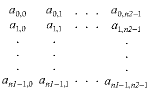
Following is a two-dimensional sequence using zero-based indexing where the first dimension is n1, and the second dimension is n2:
For the Fourier transform subroutines, a two-dimensional sequence is distributed over a one-dimensional process grid, using block-column distribution. The process grid must be arranged as a row (1 × q, where q is the number of processes).
| Note: | Two-dimensional sequences can be thought of as two-dimensional matrices. The term sequence is used because it is traditional for Fourier transforms. |
You must distribute the input sequence sequentially to the processes in the process grid, using block-column distribution. Parallel ESSL also returns the output sequence using block-column distribution. The output sequence may be returned in normal or transposed form.
A sequence can be distributed unevenly; that is, one process in the process grid can receive an array that is smaller than other processes. It can also happen that some processes receive no data. "Example 2" shows an example of uneven data distribution.
LOCq(n) represents the number of columns that a process would receive if n is distributed block over q processes. You need to calculate LOCq(n) for each process, as follows:
LOCq(n) = NB2 = (n+q-1)/q
LOCq(n) = n-(q-1)(NB2)
where:
n represents the following:
n is the second dimension, n2, of the sequence (for normal form)
n is the first dimension, n1, of the sequence (for transposed form and the sequence is not stored in FFT-packed storage mode)
n is n1/2 (for transposed form and the sequence is stored in FFT-packed storage mode)
q is the number processes in the process grid
P0,k is the process that receives the last block of data. For uneven data distribution, P0,k would receive an array that is smaller than the other processes receive.
Following is an example of block-column distribution for a two-dimensional sequence over a one-dimensional, row-oriented process grid.
Global sequence of size 8 × 12:
B,D       0            1            2             3
     *                                                   *
     |  0 10 20  |  30 40 50  |  60 70 80  |  90 100 110 |
     |  1 11 21  |  31 41 51  |  61 71 81  |  91 101 111 |
     |  2 12 22  |  32 42 52  |  62 72 82  |  92 102 112 |
     |  3 13 23  |  33 43 53  |  63 73 83  |  93 103 113 |
 0   |  4 14 24  |  34 44 54  |  64 74 84  |  94 104 114 |
     |  5 15 25  |  35 45 55  |  65 75 85  |  95 105 115 |
     |  6 16 26  |  36 46 56  |  66 76 86  |  96 106 116 |
     |  7 17 27  |  37 47 57  |  67 77 87  |  97 107 117 |
     *                                                   *
Row-oriented, 1 × 4 process grid:
| B,D | 0 | 1 | 2 | 3 |
|---|---|---|---|---|
| 0 | P00 | P01 | P02 | P03 |
Local arrays:
p,q  |     0       |      1       |      2       |      3
-----|-------------|--------------|--------------|-------------
     |  0  10  20  |  30  40  50  |  60  70  80  |  90 100 110
     |  1  11  21  |  31  41  51  |  61  71  81  |  91 101 111
     |  2  12  22  |  32  42  52  |  62  72  82  |  92 102 112
     |  3  13  23  |  33  43  53  |  63  73  83  |  93 103 113
 0   |  4  14  24  |  34  44  54  |  64  74  84  |  94 104 114
     |  5  15  25  |  35  45  55  |  65  75  85  |  95 105 115
     |  6  16  26  |  36  46  56  |  66  76  86  |  96 106 116
     |  7  17  27  |  37  47  57  |  67  77  87  |  97 107 117
An example of the distribution of a two-dimensional sequence in a Fortran 90 program is shown in Appendix B. "Sample Programs". See the following:
The output sequence for PSRCFT2 and PDRCFT2, and the input sequence for PSCRFT2 and PDCRFT2 are stored in FFT-packed storage mode because they consist of complex-conjugate, even symmetric data.
For FFT-packed storage mode, only certain elements of the complex-conjugate, even symmetric data are stored. This section describes how the complex elements of sequence y, which is the output sequence for PSRCFT2 and PDRCFT2, and the input sequence for PSCRFT2 and PDCRFT2, are stored in global matrices Y and X, respectively.
For example, suppose y is the two-dimensional sequence to be stored in FFT-packed storage mode for PDRCFT2. The following list describes how the elements in y correspond to the elements in the global matrix Y:
where:
The remaining elements of y are not stored because they are the complex conjugates of elements already stored. These relationships are shown in the following equations:
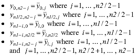
where:
The following example, which uses zero-based indexing, has complex conjugate, even symmetry. The dimensions of array y are 8 × 8 (that is n1 = n2 = 8), where array y is:
    *                                                                         *
    | (111,0)  (-3,23)  (-8,10)   (-9,4)   (-9,0)  (-9,-4)  (-8,-10)  (-3,-23)|
    |(10,-10)    (4,4)    (9,3)   (-6,2)   (-1,2)   (-2,1)    (-3,1)   (-5,-3)|
    |  (6,-4)    (1,3)    (0,2)   (-7,1)   (-1,9)   (-1,4)   (-2,-4)   (-2,-2)|
    |  (6,-2)    (6,2)   (-5,1)   (-8,8)   (-1,4)  (-1,-1)   (-1,-8)   (-1,-2)|
    |   (6,0)   (-3,2)   (-9,1)   (-1,5)   (-1,0)  (-1,-5)   (-9,-1)   (-3,-2)|
    |   (6,2)   (-1,2)   (-1,8)   (-1,1)  (-1,-4)  (-8,-8)   (-5,-1)    (6,-2)|
    |   (6,4)   (-2,2)   (-2,4)  (-1,-4)  (-1,-9)  (-7,-1)    (0,-2)    (1,-3)|
    | (10,10)   (-5,3)  (-3,-1)  (-2,-1)  (-1,-2)  (-6,-2)    (9,-3)    (4,-4)|
    *                                                                         *
Because zero-based indexing is used, y0,0 = (111,0), y3,2 = (-5,1), and y5,7 = (6,-2).
In this example, the real part of y0,0 is 111, the real part of y0,4 is-9, the real part of y4,0 is 6, the real part of y4,4 is-1, and their imaginary parts are all zero. For the FFT-packed storage mode, the imaginary parts at these particular positions are not stored. Therefore, the number stored at position Y0,0 is (111,-9), which represents the contents of both y0,0 and y0,4. The number stored at position Y4,0 is (6,-1), which represents the contents of both y4,0 and y4,4.
The elements y0,1:3 are stored in Y1:3,0. The elements y4,1:3 are stored in Y5:7,0. The rows y1:3,0:7 are stored in columns Y0:7,1:3. For FFT-packed storage mode, the elements in positions y0,5:7, y4,5:7, and rows y5:7,0:7 are not stored.
Following is the global matrix Y in FFT-packed storage mode:
B,D            0                    1
     *                                        *
     | (111,-9) (10,-10)  |   (6,-4)   (6,-2) |
     |  (-3,23)  (4,  4)  |   (1, 3)   (6, 2) |
     |  (-8,10)  (9,  3)  |   (0, 2)  (-5, 1) |
     |  (-9, 4) (-6,  2)  |  (-7, 1)  (-8, 8) |
 0   |   (6,-1) (-1,  2)  |  (-1, 9)  (-1, 4) |
     |  (-3, 2) (-2,  1)  |  (-1, 4)  (-1,-1) |
     |  (-9, 1) (-3,  1)  |  (-2,-4)  (-1,-8) |
     |  (-1, 5) (-5, -3)  |  (-2,-2)  (-1,-2) |
     *                                        *
Following is a 1 × 2 process grid:
| B,D | 0 | 1 |
|---|---|---|
| 0 | P00 | P01 |
After the data has been distributed over the process grid, the following local arrays for Y are stored in FFT-packed storage mode:
p,q  |         0           |         1
-----|---------------------|-------------------
     | (111,-9)  (10,-10)  |   (6,-4)   (6,-2)
     |  (-3,23)   (4,  4)  |   (1, 3)   (6, 2)
     |  (-8,10)   (9,  3)  |   (0, 2)  (-5, 1)
     |  (-9, 4)  (-6,  2)  |  (-7, 1)  (-8, 8)
 0   |   (6,-1)  (-1,  2)  |  (-1, 9)  (-1,4)
     |  (-3, 2)  (-2,  1)  |  (-1, 4)  (-1,-1)
     |  (-9, 1)  (-3,  1)  |  (-2,-4)  (-1,-8)
     |  (-1, 5)  (-5, -3)  |  (-2,-2)  (-1,-2)
The following example shows how to pack data from a two-dimensional array X into a global array XG, whose columns could then be block-column distributed among q processes. Array X must contain complex-conjugate even symmetric data.
Each of the q processes would get LOCq(n) consecutive columns of array XG. Array X is stored as n1 rows by n2 columns. Array XG is stored as n2 rows by n1/2 columns. This is the transposed form required by PSCRFT2 and PDCRFT2 for the input array.
     PROGRAM PACK2D
     IMPLICIT NONE
     INTEGER*4 N1,N2,INDEX,JINDEX
     PARAMETER(N1 = 64, N2 = 32)
     COMPLEX*16 XG(0:N2-1,0:N1/2-1)
     COMPLEX*16 X(0:N1-1,0:N2-1)
     XG(0,0)    = ( REAL(X(0,0))    , REAL(X(0,N2/2))    )
     XG(N2/2,0) = ( REAL(X(N1/2,0)) , REAL(X(N1/2,N2/2)) )
     DO INDEX = 1 , N2/2-1
        XG(INDEX,0) = X(0,INDEX)
        XG(N2/2+INDEX,0) = X(N1/2,INDEX)
     ENDDO
     DO JINDEX = 0,N2-1
      DO INDEX = 1,N1/2-1
         XG(JINDEX,INDEX) = X(INDEX,JINDEX)
      ENDDO
     ENDDO
     STOP
     END
Following is a three-dimensional sequence using zero-based indexing where the first dimension is n1, the second dimension is n2, and the third dimension is n3:
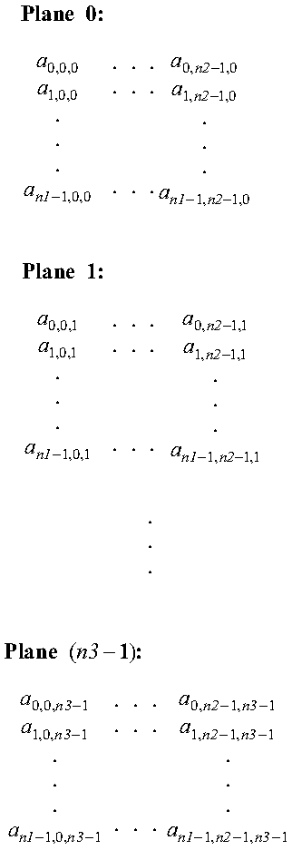
For the Fourier transform subroutines, a three-dimensional sequence is distributed over a one-dimensional process grid, using block-plane distribution. The process grid must be arranged as a row (1 × q, where q is the number of processes).
| Note: | Three-dimensional sequences can be thought of as three-dimensional matrices. The term sequence is used because it is traditional for Fourier transforms. |
You must distribute the three-dimensional input sequence sequentially to the processes in the process grid, using block-plane distribution. Parallel ESSL also returns the output sequence using block-plane distribution. The output sequence may be returned in normal or transposed form.
A sequence can be distributed unevenly; that is, one process in the process grid can receive an array that is smaller than other processes. It can also happen that some processes receive no data. "Example 2" shows an example of when a process does not receive any data.
LOCq(n) represents the number of planes that a process would receive if n is distributed block over q processes. You need to calculate LOCq(n) for each process, as follows:
LOCq(n) = NB3 = (n+q-1)/q
LOCq(n) = n-(q-1)(NB3)
where:
n represents the following:
n is the third dimension, n3, of the sequence (for normal form)
n is the first dimension, n1, of the sequence (for transposed form and the sequence is not stored in FFT-packed storage mode)
n is n1/2 (for transposed form and the sequence is stored in FFT-packed storage mode)
q is the number processes in the process grid
P0,k is the process that receives the last block of data. For uneven data distribution, P0,k would receive an array that is smaller than the other processes receive.
Following is an example of block plane distribution for a three-dimensional sequence over a one-dimensional process grid.
Three-dimensional, global sequence with four planes that are of size 2 × 2:
        Plane 0:      Plane 1:
----------------------------------------------
B,D               0
----------------------------------------------
     *                          *
 0   |    0  1    |    10 101   |
     |   10 11    |    11 111   |
     *                          *

        Plane 2:      Plane 3:
----------------------------------------------
B,D               1
----------------------------------------------
     *                          *
 0   |   20 21    |    30 31    |
     |   23 24    |    33 34    |
     *                          *
Row-oriented, 1 × 2 process grid:
| B,D | 0 | 1 |
|---|---|---|
| 0 | P00 | P01 |
Local arrays:
p,q  |       0        |       1
-----|----------------|---------------
 0   |  0  1  10 101  |  20 21  30 31
     | 10 11  11 111  |  23 24  33 34
The output sequence for PSRCFT3 and PDRCFT3, and the input sequence for PSCRFT3 and PDCRFT3 are stored in FFT-packed storage mode because they consist of complex-conjugate, even symmetric data.
For FFT-packed storage mode, only certain elements of the complex-conjugate, even symmetric data are stored. This section describes how the complex elements of sequence y, which is the output sequence for PSRCFT3 and PDRCFT3, and the input sequence for PSCRFT3 and PDCRFT3, are stored in global matrices Y and X, respectively.
For example, suppose y is the three-dimensional sequence to be stored in FFT-packed storage mode for PDRCFT3. The following list describes how the elements in y correspond to the complex elements in the global matrix Y:
where:
The remaining elements of y are not stored because they are the complex conjugates of elements already stored. These relationships are shown in the following equations:
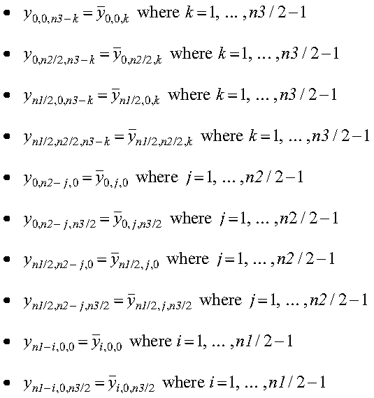
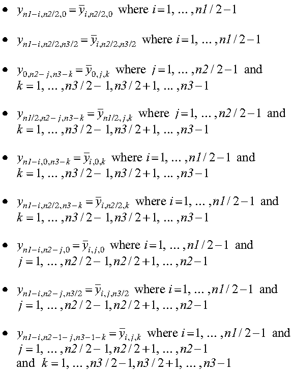
where:
The following example, which uses zero-based indexing, has complex-conjugate, even symmetry. The dimensions of array y are 4 × 4 × 4 (that is n1 = n2 = n3 = 4).
Plane 0:
y0:3,0:3,0 =
             *                                             *
             |     (30,0)     (2,-3)   (-0.3,0)     (2,3)  |
             |   (-1,0.7)    (-1,-4)  (-2,-0.7)  (0.5,-2)  |
             |     (-2,0)  (-2,-0.6)      (2,0)  (-2,0.6)  |
             |  (-1,-0.7)    (0.5,2)   (-2,0.7)    (-1,4)  |
             *                                             *
Plane 1:
y0:3,0:3,1 =
             *                                                 *
             |    (2,-2)       (-1,1)   (0.7,-2)      (-3,-2)  |
             |     (2,2)      (-2,-1)   (-0.5,3)   (0.04,0.5)  |
             |  (-0.4,3)  (-0.009,-3)  (0.9,0.1)    (-1,-0.2)  |
             |   (-2,-2)      (-2,-1)   (-0.5,2)  (0.1,0.005)  |
             *                                                 *
Plane 2:
y0:3,0:3,2 =
             *                                             *
             |      (3,0)  (0.3,0.5)  (0.1,0)  (0.3,-0.5)  |
             |  (-0.3,-2)     (1,-3)    (2,3)      (-7,3)  |
             |      (2,0)     (2,-1)    (1,0)       (2,1)  |
             |   (-0.3,2)  (-0.7,-3)   (2,-3)       (1,3)  |
             *                                             *
Plane 3:
y0:3,0:3,3 =
             *                                                  *
             |      (2,2)       (-3,2)     (0.7,2)     (-1,-1)  |
             |     (-2,2)   (1,-0.005)   (-0.5,-2)    (-0.2,1)  |
             |  (-0.4,-3)     (-1,0.2)  (0.9,-0.1)  (-0.009,3)  |
             |     (2,-2)  (0.04,-0.5)   (-0.5,-3)      (-2,1)  |
             *                                                  *
Because zero-based indexing is used, y0,0,0 = (30,0), y2,1,1 = (-0.009,-3), and y3,1,3 = (0.04,-0.5).
In this example, the real part of y0,0,0 is 30, the real part of y0,0,2 is 3, and their imaginary parts are zero. For the FFT-packed storage mode, the imaginary parts at these particular positions are not stored. Therefore, the element stored at position Y0,0,0 is (30,3), which represents the contents of both y0,0,0 and y0,0,2.
The element y0,0,1 is stored in the global matrix Y1,0,0 position.
The real part of y0,2,0 is-0.3, the real part of y0,2,2 is 0.1, and their imaginary parts are zero. For the FFT-packed storage mode, the imaginary parts at these particular positions are not stored. Therefore, the element stored at position Y2,0,0 is (-0.3,0.1), which represents the contents of both y0,2,0 and y0,2,2.
The element y0,2,1 is stored in the global matrix Y3,0,0 position.
The real part of y2,0,0 is-2, the real part of y2,0,2 is 2, and their imaginary parts are zero. For the FFT-packed storage mode, the imaginary parts at these particular positions are not stored. Therefore, the element stored at position Y0,2,0 is (-2,2), which represents the contents of both y2,0,0 and y2,0,2.
The element y2,0,1 is stored in the global matrix Y1,2,0 position.
The real part of y2,2,0 is 2, the real part of y2,2,2 is 1, and their imaginary parts are zero. For the FFT-packed storage mode, the imaginary parts at these particular positions are not stored. Therefore, the element stored at position Y2,2,0 is (2,1), which represents the contents of both y2,2,0 and y2,2,2.
The element y2,2,1 is stored in the global matrix Y3,2,0 position.
The rows y0,1,0:3 are stored in columns Y0:3,1,0. The rows y2,1,0:3 are stored in columns Y0:3,3,0. The plane y1,0:3,0:3 is stored in plane Y0:3,0:3,1. For FFT-packed storage mode, the remaining elements do not need to be stored due to symmetry.
Following is the global matrix Y in FFT-packed storage mode:
Plane 0:
B,D                             0
     *                                                     *
     |    (30,  3)     (2,  -3)      (-2, 2)    (-2, -0.6) |
     |     (2, -2)     (-1,  1)     (-0.4,3)   (-0.009,-3) |
 0   | (-0.3, 0.1)   (0.3, 0.5)      (2,  1)       (2,  1) |
     |   (0.7, -2)      (-3, 2)   (0.9, 0.1)     (-1, 0.2) |
     *                                                     *
Plane 1:
B,D                             1
     *                                                      *
     |  (-1,0.7)        (-1, -4)   (-2, -0.7)     (0.5, -2) |
     |     (2,2)         (-2,-1)    (-0.5, 3)   (0.04, 0.5) |
 0   | (-0.3,-2)         (1, -3)      (2,  3)     (-0.7, 3) |
     |   (-2, 2)  (-0.1, -0.005)   (-0.5, -2)     (-0.2, 1) |
     *                                                      *
Following is a 1 × 2 process grid:
| B,D | 0 | 1 |
|---|---|---|
| 0 | P00 | P01 |
After the data has been distributed over the process grid, the following local arrays for Y are stored in FFT-packed storage mode:
p,q  |                       0                        |                         1
-----|------------------------------------------------|--------------------------------------------------
     |    (30,  3)   (2,  -3)    (-2, 2)  (-2, -0.6)  |   (-1,0.7)       (-1, -4) (-2, -0.7)   (0.5, -2)
     |     (2, -2)   (-1,  1)   (-0.4,3) (-0.009,-3)  |      (2,2)        (-2,-1)  (-0.5, 3) (0.04, 0.5)
 0   | (-0.3, 0.1) (0.3, 0.5)    (2,  1)     (2,  1)  |  (-0.3,-2)        (1, -3)    (2,  3)   (-0.7, 3)
     |   (0.7, -2)    (-3, 2) (0.9, 0.1)   (-1, 0.2)  |    (-2, 2) (-0.1, -0.005) (-0.5, -2)   (-0.2, 1)
The following example shows how to pack data from a three-dimensional array X into a global array XG, whose planes could then be block distributed among q processes. Array X must contain complex-conjugate even symmetric data.
Each of the q processes would get LOCq(n) consecutive planes of array XG. Array X is stored as n1 rows by n2 columns by n3 planes. Array XG is stored as n3 rows by n2 columns by n1/2 planes. This is the transposed form required by PSCRFT3 and PDCRFT3 for the input array. n1, n2, and n3 are divisible by 2q, as required by PSCRFT3 and PDCRFT3.
     PROGRAM PACK3D
     IMPLICIT NONE
     INTEGER*4 N1,N2,N3
     INTEGER*4 IINDEX,JINDEX,KINDEX
     PARAMETER(N1 = 64, N2 = 32, N3 = 48)
     COMPLEX*16 XG(0:N3-1,0:N2-1,0:N1/2-1)
     COMPLEX*16 X(0:N1-1,0:N2-1,0:N3-1)
     XG(0,0,0)    = ( REAL(X(0,0,0))    , REAL(X(0,0,N3/2))    )
     XG(N3/2,0,0) = ( REAL(X(0,N2/2,0)) , REAL(X(0,N2/2,N3/2)) )
     XG(0,N2/2,0) = ( REAL(X(N1/2,0,0)) , REAL(X(N1/2,0,N3/2)) )
     XG(N3/2,N2/2,0) = (REAL(X(N1/2,N2/2,0)),REAL(X(N1/2,N2/2,N3/2)))
     DO IINDEX = 1 , N3/2-1
        XG(IINDEX,0,0) = X(0,0,IINDEX)
        XG(N3/2+IINDEX,0,0) = X(0,N2/2,IINDEX)
        XG(IINDEX,N2/2,0) = X(N1/2,0,IINDEX)
        XG(N3/2+IINDEX,N2/2,0) = X(N1/2,N2/2,IINDEX)
     ENDDO
     DO KINDEX = 0,N3-1
      DO JINDEX = 1,N2/2-1
        XG(KINDEX,JINDEX,0) = X(0,JINDEX,KINDEX)
        XG(KINDEX,N2/2+JINDEX,0) = X(N1/2,JINDEX,KINDEX)
      ENDDO
     ENDDO
     DO KINDEX = 0,N3-1
      DO JINDEX = 0,N2-1
       DO  IINDEX = 1,N1/2-1
          XG(KINDEX,JINDEX,IINDEX) = X(IINDEX,JINDEX,KINDEX)
       ENDDO
      ENDDO
     ENDDO
     STOP
     END