l1
A1x1 = b ;
The modeling phase includes:
The solver phase includes:
The analysis of solution data is a complex issue. The number of ways the user can implement the functions of the IBM Optimization Library Stochastic Extensions is so great that it is difficult to anticipate all possible user requirements. The Solver provides access to:
The callable modules provide complete access to all solution data, including dual information.
All information concerning a particular instance of a stochastic program is organized as a structured data type called Stoch_Data. This structure is initialized by a call to subroutine ekks_InitializeApplication, which returns a pointer to the Stoch_Data data type. Every Callable Module uses this pointer to access the data of the stochastic program. Multiple instances of stochastic programs can appear in the same program module, each with their own unique Stoch_Data pointer.
The generic IBM Stochastic Extensions driver consists of five subroutine calls:
     #include "ekkstoch.h"
     Stoch_Data *stoch_data;
         ekk_Initialize();
     ekks_InitializeApplication(&rc,&stoch_data,...);
     ekks_CreateCore(&rc,stoch_data,... );
     for(s=0;s<max_s;s++)
     {
         ekks_AddScenario(&rc,stoch_data,s,...);
     }
     ekks_BendersLSolve(&rc,stoch_data,osl_dspace,...);
     for(s=0;s<max_s;s++)
     {
         ekks_GetSolution(&rc,stoch_data,s,soln,...);
         printf( ... , soln);
     }
The call to ekks_InitializeApplication
initializes the stoch_data pointer to the Stoch_Data
object. The calls to ekks_CreateCore
(declare core file) and ekks_AddScenario
(add a scenario) pass the problem data to the Stoch_Data object.
A call to ekks_BendersLSolve
declares and solves the stochastic problem with a Benders decomposition
method implemented in the IBM Optimization Library
subroutines. The subroutine ekks_GetSolution
accesses scenario solutions one-by-one after which they may be processed
by the user (for example, printed).
Scenario data is defined relative to the core data. For details of this convention, see the documentation of the ekks_AddScenario subroutine.
SPL-file storage is managed by IBM Stochastic Extensions I/O routines. Users have access to this information through special purpose data-access routines. The SP-file may be saved (ekks_PutStochasticData), in which case it will contain all information necessary to restore (ekks_GetStochasticData) the stochastic program.
The data required for the definition of a stochastic program is organized
into a structure of type Stoch_Model. A Stoch_Model can
be thought of as a selection of a subset of nodes from a Stoch_Data.
(They are not the same sort of structure, since the node data for the submodel
is obtained by reference to the original Stoch_Data structure.)
A stochastic model is created by passing a list of nodes to the
appropriates IBM Stochastic Extensions subroutine ekks_DescribeModel.
By default, a Stoch_Data structure is considered to be itself
a stochastic model containing all possible nodes.
The data pointed to by the structures Stoch_Data and Stoch_Model is internal and protected from the user. But all stochastic programming data is available to the user via the structures usrCoreData, usrStoch, usrNode, and usrNodeData, as referenced in the Data Structures Reference. These must be filled by special subroutine calls using: ekks_GetCoreData, ekks_GetScenarioTree and/or ekks_GetNodeData. The sample driver programs exsdst.c, and exsolv.c show examples of user data access.
Calls to user access subroutines can have a Stoch_Data or a Stoch_Model pointer in the argument list. In the latter case, the list of nodes returned will be those that appeared in the model's original list, plus the list of appropriately marked virtual nodes. Offsets and probabilities refer to the relevant model.
The node data retrieved by a call to ekks_GetNodeData
contains only the stochastic data. It must be combined with the appropriate
core data obtained by ekks_GetCoreData.
It is important to note is that the data may have been sorted during the
input phase. Particular items may have been moved out of their original
positions. The usrCoreData
structure has pointers to the sort keys used to translate the row and column
indices from external (i.e. user) order to internal, and back.
minimize x1 c1T x1 + E2 Q2( x1 ) ,
subject to:
x1 ![]()
![]() n1 ,
n1 ,
l1
![]() x1
x1
![]() u1 ,
u1 ,
A1x1 = b ;
where the functions Q2, Q3, ... , QT are defined recursively by:
Q2( x1 )
= minx2
c2T
x2 + E3 Q3( x1 , x2 ) ,
subject to:
x2 ![]()
![]() n2 ,
n2 ,
l2
![]() x2
x2 ![]() u2 ,
u2 ,
A2, 1 x1
+ A2, 2 x2
= b2 ,
Q3( x1 , x2 )
= minx3
c3T
x3 + E4 Q4( x1 , x2 ,
x3 ) ,
subject to:
x2 ![]()
![]() n3 ,
n3 ,
l3 ![]() x3
x3 ![]() u3 ,
u3 ,
A3, 1 x1
+ A3, 2 x2
+ A3, 3 x3
= b3 ,
and so on, for Qt , t = 4, ... , T - 1. In each of the forgoing equations, "Et" represents the expectation with respect to the random variables in period number t . Finally, QT is defined by:
QT ( x1, ... , xT-1 ) = minxT
cTT
xT ,
subject to:
x2 ![]()
![]() nT ,
nT ,
lT ![]() xT
xT ![]() uT ,
uT ,
AT, 1 x1
+ AT, 2 x2
+ ... +
AT, T xT
= bT .
The data defining this problem may be arranged in a LP formulation for a single realization of the random variables:
objective: STj=1 ctT xt ,
constraints:
xt ![]()
![]() nt
for t = 1, ... , T ,
nt
for t = 1, ... , T ,
lt ![]() xt
xt ![]() ut
for t = 1, ... , T ,
ut
for t = 1, ... , T ,
A1x1
= b1 ![]()
![]() m1 , and
m1 , and
Stj=1
At , j xj
= bt ![]()
![]() mt
, for t = 2, ... , T .
mt
, for t = 2, ... , T .
All entries of the matrices At , j and vectors: ct , lt ,
ut , bt may be random (although in
practice all but a few entries will be deterministic). The indices t
= 1, ... ,T signify the periods of the problem; to each period t
there corresponds a decision vector xt ![]()
![]() nt.
The lower block-triangular constraint system expresses the typical feature
of these problems--the decisions of the prior periods constrain the decision
of the current period explicitly (since those decisions are known) but the
decision of the current period is affected only implicitly by the feasibility
and costs of possible future (recourse) decisions.
nt.
The lower block-triangular constraint system expresses the typical feature
of these problems--the decisions of the prior periods constrain the decision
of the current period explicitly (since those decisions are known) but the
decision of the current period is affected only implicitly by the feasibility
and costs of possible future (recourse) decisions.
The proposed format is most easily understood by considering the above multistage LP in stages of gradually increasing levels of detail. First we regard it as a purely deterministic problem and create an input file following the MPS convention, ignoring (non-random) zero entries. This file will identify an objective vector, upper and lower bounds, a right hand side, and a block lower-triangular matrix, all expressed in the usual column-row format; we call this the core file.
Next we note the period structure of the problem, that certain decisions are made at certain times. Here it is necessary only to specify which rows and columns from the core file correspond to which periods. It is most simply done by indicating the beginning column and row for each period. This is done in the time file. Such a system relies on the proper sequencing of the core file--we require that the list of row names is in order from first period to last period and that the block lower-triangular matrix has been entered in column order: first period columns first, and last period columns last.
Finally there remains the specification of the distributions of the random entries; this takes place in the stoch file. The simplest case occurs when all random entries are mutually independent. We consider two general types of dependency among the random entries: blocks and scenarios. A block is a random vector whose realizations are observed in a single, fixed period. A scenario is a more general type of stochastic structure which models dependencies across periods.
The organization of the data files is similar to the MPS format. Each data file contains a number of sections, some of which are optional. A header line, or header, marks the beginning of each section and may contain keywords to inform the user that the data to follow should be treated in a special way. Each header line is divided into two fields delimited by specific columns.
1...5.........15........25.............40........50.............
NAME          problem name
* this is a comment line
ROWS
 N  OBJ
 L  ROW1
 E  ROW2
    -etc-
COLUMNS
1...5.........15........25.............40........50.............
    COL1      ROW1      value          ROW2      value
    COL1      ROW3      value          ROW4      value
    -etc-
    RHS
    RHS       ROW1      value          ROW2      value
    -etc-
BOUNDS
 LO BND       COL1      value
    -etc-
RANGES
    -etc-
ENDATA
Integer variables may be indicated by using delimiters as described in the MPS/MIP standard. for those users who want to use mixed integer programming techniques.(1)
1...5.........15........25.............40........50.............
TIME          problem name
PERIODS
    COL1      ROW1                     PERIOD1
    COL6      ROW3                     PERIOD2
    COL8      ROW19                    PERIOD3
ENDATA
In this example: Columns COL1 through COL5 are PERIOD1 decision variables and COL6 and COL7 are PERIOD2 variables; rows ROW1 and ROW2 are PERIOD1 constraints and ROW3 through ROW18 are PERIOD2 constraints. All remaining rows and columns belong to PERIOD3.
1...5.........15........25.............40........50.............
INDEP         DISCRETE
    COL1      ROW8      6.0            PERIOD2   0.5
    COL1      ROW8      8.0            PERIOD2   0.5
    RHS       ROW8      1.0            PERIOD2   0.1
    RHS       ROW8      2.0            PERIOD2   0.5
    RHS       ROW8      3.0            PERIOD2   0.4
In this example the entry COL1/ROW8 takes value 6.0 with probability 0.5 and 8.0 with probability 0.5; and the right hand side of ROW8 takes values (1.0,2.0,3.0) with probabilities (0.1,0.5,0.4) respectively. Of course the probabilities associated with an entry must total one.
1...5.........15........25.............40........50.............
INDEP         UNIFORM
    COL1      ROW8      8.0            PERIOD2   9.0
In this example the random entry COL1/ROW8 is uniformly distributed over the interval [8.0, 9.0].
1...5.........15........25.............40........50.............
INDEP         NORMAL
    COL1      ROW8      0.0            PERIOD2   1.0
In this example the random variable is normal with mean 0.0 and variance 1.0.
1...5.........15........25.............40........50.............
BLOCKS        DISCRETE
 BL BLOCK1    PERIOD2   0.5
    COL1      ROW6      83.0
    COL2      ROW8      1.2
 BL BLOCK1    PERIOD2   0.2
    COL1      ROW6      83.0
    COL2      ROW8      1.3
 BL BLOCK1    PERIOD2   0.3
    COL1      ROW6      84.0
    COL2      ROW8      1.2
ENDATA
In this example the block, called BLOCK1, is the vector made up of the entries COL1/ROW6 and COL2/ROW8. It takes values (83.0,1.2) with probability 0.5, (83.0,1.3) with probability 0.2, and (84.0,1.2) with probability 0.3.
1...5.........15........25.............40........50.............
BLOCKS        LINTR
 BL V_BLOCK   PERIOD2
    COL1      ROW8
    COL3      ROW6
 RV U1        NORMAL    0.0                      1.0
    COL1      ROW8      11.0
    COL3      ROW6      21.0
 RV U2        UNIFORM   -1.0                     1.0
    COL1      ROW8      12.0
    COL3      ROW6      22.0
 RV U3        CONSTANT
    COL3      ROW6      24.0
This example illustrates the file structure. In this case
Note that the "names" U1, U2 and U3 are irrelevant and may be left blank.
To describe the process paths in the discrete state case, note that process can assume only finitely many values. A path of the process up to a given time stage may be followed by a finite collection of possible values of the process in the next time period. We think of these as nodes in the next period. Following Lane and Hutchinson and Raiffa, we construct an event tree representation of the trajectories: Represent the (unique) value of the process in the first period by a single node connected by oriented arcs from that node to nodes representing the values of the process in period 2. These are the descendant nodes of the first period node in the terminology of Birge. Each node of period 2 is connected to its descendant nodes at period 3 by individual arcs oriented in the direction of the period 3 nodes. This construction is continued by connecting each ancestor with its descendant nodes in the next period. Each node of this tree has a single entering arc and multiple departing arcs representing the possible next period events.
A single trajectory of the process thus corresponds to a path from the period 1 node to a single period T node composed of arcs oriented in the direction of increasing time, and moreover, corresponds uniquely to a single node in the last period T. There are only finitely many paths linking nodes in period 1 to nodes in period T, and to specify the distribution on the paths one needs only to attach a definite probability to each path. Hence specifying the process distribution in terms of path probabilities can be effected in this context by assigning probabilities to period T nodes of the hyperreferent tree event tree, see Figure 1.1 below.
The topology of this event tree represents the information about the process. To each arc we attach the probability that the terminal node occurs given the initial node has occurred--that is, the conditional probability of the process distribution over a period conditional on the history over all previous periods. These arc probabilities can be computed from the path probabilities by summing the probabilities of the paths visiting the terminal node, and then dividing by the sum of the probabilities of the paths visiting the initial node.
Conversely, if to each arc in the tree we know the conditional probability that its terminal node occurs given that its initial node has occurred, then the probability of any given path is simply the product of the arc probabilities along the path.
A decision at a given node is made only on the basis of information collected up to and including that node. The uncertainty faced by the decision maker is
represented by the collection of paths that branch from this node. Thus in the following Figure, the decisions occur at the nodes
and the scenarios branch after the node.
|
In a language more specific to our application, a "path" in the tree analogy is a single "scenario". The nodes visited by the path correspond to certain values assumed by certain entries of the matrices in the core file. Thus a scenario is completely specified by a list of column/row names and values, and a probability value. Once a single given scenario is described, then other scenarios that branch from it may be described by indicating in which period the branch has occurred, and then listing the subsequent column/row names and values. It is best to work through the example shown in the preceding Figure.
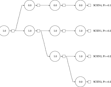
There are two types of data lines. The first, signified by SC in the code field, gives the name of the scenario in the first name field and its probability in the first numeric field, and then gives the name of the scenario from which the branch occurred and the name of the period in which the branch occurred --i.e., the first period in which the two scenarios differ-- in the second and third name fields, respectively. A scenario that originates in period one is indicated by ROOT in the name field. The next data lines give the column/row values assumed by the scenario.
1...5.........15........25.............40........50.............
SCENARIOS     DISCRETE
 SC SCEN1     ROOT      0.5            PERIOD1
    COL1      ROW2      1.0
    COL2      ROW3      1.0
    COL3      ROW4      1.0
    COL4      ROW5      1.0
 SC SCEN2     SCEN1     0.2            PERIOD3
    COL3      ROW4      1.0
    COL4      ROW5      1.0
 SC SCEN3     SCEN2     0.2            PERIOD4
    COL4      ROW5      0.0
 SC SCEN4     SCEN1     0.1            PERIOD2
    COL2      ROW3      0.0
    COL3      ROW4      0.0
    COL4      ROW5      0.0
ENDATA
This is a description of the distribution of four entries: COL1/ROW2, COL2/ROW3, COL3/ROW4, COL4/ROW5, which for convenience we denote here as d1, d2, d3, and d4, respectively. Note that in PERIOD4 there are two nodes for the "state" d4 equals 0.0 and two for d4 equals 1.0, and similarly in PERIOD3 two nodes for d3 equals 1.0. This is because a node is distinguished by the information that one has collected concerning the path up to and including that node. Thus in PERIOD3 the two nodes are distinguished because in scenario SCEN1 one knows that the final state is d4 equals 1.0, whereas in SCEN2 the outcome of d4 is in doubt.
The solution procedure consists of a nested L-shaped, or Benders, decomposition phase, and if needed, a Simplex method phase. The decomposition may not terminate in a reasonable number of iterations, for this reason it is often useful to follow Benders with the Simplex method. This is automatically done if the number of major cycles exceeds Benders_Major_Iterations.
In the decomposition phase, the problem is decomposed into subproblems according to one of several user-specified criteria: Problem_Size, Maximum_Subproblems, or Cut_Stage.
If there are more subproblems than the maximum number of subproblems allowed, Maximum_Subproblems, then the subtrees are divided among the subproblems as evenly as possible. In the case of a cut at a time stage Cut_Stage, the first subproblem is joined to the master problem, thus the master consists of the nodes less than Cut_Stage together with the subtrees collected into the first subproblem. This "augmented master" tends to produce better proposals; for example, the master nodes might be unbounded without the influence of some downstream nodes. If the tree is not decomposed by time stage, then no augmented master is generated.
In nested decomposition, subproblems can generate both cuts and proposals, depending on their position in the subproblem tree. The implementation requires that all child subproblems report OPTIMAL before the subproblem will generate a cut for its parent, and that a subproblem generates a proposal for its children only when it has received a new proposal from its parent. (This is the so-called Fast Forward, Fast Back protocol.) Only optimal cuts and proposals are generated.
Changing the number Maximum_Subproblems can have a big effect on the performance of Benders decomposition. For example, 100 subproblems will generate 100 different cuts, whereas 1 subproblem will generate 1 cut from the same proposal. The difference is the level of aggregation: the 1 cut from 1 subproblem is in fact the aggregation of the 100 cuts from the 100 subproblems. Generally speaking, aggregated cuts contain less information than the collection of disaggregated cuts, but disaggregated cuts make the master problem grow much faster.
Major iterations of Benders decomposition are performed until either a relative optimality gap of size less than Optimality_Gap is attained, or the maximum number of iterations Benders_Major_Iterations is performed. A major iteration consists of:
Experience suggests that the solution progress is most affected by the Problem_Size and the maximum number of major iterations. Large subproblems take a long time to solve. A large number of small subproblems will spend a long time resolving root proposals.
Those parameters not yet described affect to the solution procedures applied within the Benders decomposition. These procedures are implemented in IBM Optimization Library subroutines, and the parameters refer to the calling sequences of these subroutines, which are documented in the Optimization Library Users Guide and Reference. A method or type setting of zero means that the procedure will not be called. For example, the parameter EKKCRSH_method refers to the parameter passed to EKKCRSH, which is called at the initial solution of any subproblem, master or subproblem. If this parameter is set to zero, then EKKCRSH would not be called (not recommended!). The actual instantiation is if (icrsh) ekkcrsh(iret,osl_dspace,icrsh);, and similarly for the other procedures.
[ Top of Page | Previous (Roadmap) | Next (Reference Section) | Table of Contents ]