Guide and Reference
- Doing extrapolation with SPINT and DPINT is not encouraged unless you know
the consequences of doing polynomial extrapolation.
- If performance is the overriding consideration, you should investigate
using the general signal processing subroutines, DQINT and SQINT.
- There are some ESSL-specific rules that apply to the results of
computations on the workstation processors using the ANSI/IEEE standards. For
details, see "What Data Type Standards Are Used by ESSL, and What Exceptions Should You Know About?".
This section contains the interpolation subroutine descriptions.
These subroutines compute the Newton divided difference coefficients and
perform a polynomial interpolation through a set of data points at specified
abscissas.
Table 150. Data Types
| x, y, c, t, s
| Subroutine
|
| Short-precision real
| SPINT
|
| Long-precision real
| DPINT
|
| Fortran
| CALL SPINT | DPINT (x, y, n, c,
ninit, t, s, m)
|
| C and C++
| spint | dpint (x, y, n, c,
ninit, t, s, m);
|
| PL/I
| CALL SPINT | DPINT (x, y, n, c,
ninit, t, s, m);
|
- x
- is the vector x of length n, containing the abscissas
of the data points used in the interpolations. The elements of x
must be distinct. Specified as: a one-dimensional array of (at least)
length n, containing numbers of the data type indicated in Table 150.
- y
- is the vector y of length n, containing the ordinates
of the data points used in the interpolations. Specified as: a
one-dimensional array of (at least) length n, containing numbers of
the data type indicated in Table 150.
- n
- is the number of elements in vectors x, y, and
c--that is, the number of data points. Specified as: a
fullword integer; n >= 0.
- c
- is the vector c of length n, where:
If ninit <= 0, all elements of c are
undefined on entry.
If ninit > 0, c contains the Newton divided
difference coefficients, cj for
j = 1, ninit, for the interpolating polynomial
through the data points
(xj,yj) for
j = 1, ninit. If
ninit < n, the values of
cj for j = ninit+1,
n are undefined.
Specified as: a one-dimensional array of (at least) length
n, containing numbers of the data type indicated in Table 150.
- ninit
- indicates the following:
If ninit <= 0, this is the first call to this subroutine
with the data in x and y; therefore, none of the Newton
divided difference coefficients in c have been initialized.
If ninit > 0, a previous call to this subroutine was
made with the data points (xj,
yj) for j = 1, ninit,
where:
- If ninit = n, all the Newton divided difference
coefficients in c were computed for the data points. No additional
coefficients are computed on this entry.
- If ninit < n, the first ninit Newton
divided difference coefficients in c were computed for the data
points (xj, yj) for
j = 1, ninit. The coefficients are updated for the
additional data points (xj,
yj) for j = ninit+1,
n on this entry.
Specified as: a fullword integer;
ninit <= n.
- t
- is the vector t of length m, containing the abscissas
at which interpolation is to be done. Specified as: a one-dimensional
array of (at least) length m, containing numbers of the data type
indicated in Table 150.
- s
- See 'On Return'.
- m
- is the number of elements in vectors t and
s--that is, the number of interpolations to be performed.
Specified as: a fullword integer; m >= 0.
- c
- is the vector c of length n, containing the
coefficients of the Newton divided difference form of the interpolating
polynomial through the data points
(xj,yj) for
j = 1, n. Returned as: a one-dimensional array
of (at least) length n, containing numbers of the data type indicated
in Table 150.
- ninit
- is the number of coefficients, n, in output vector c.
(If you call this subroutine again with the same data, this value should be
specified for ninit.) Returned as: a fullword integer;
ninit = n.
- s
- is the vector s of length m, containing the resulting
interpolated values; that is, each si is the
value of the interpolating polynomial evaluated at
ti. Returned as: a one-dimensional array of
(at least) length m, containing numbers of the data type indicated in
Table 150.
- In your C program, argument ninit must be passed by reference.
- Vectors x, y, and t must have no common elements
with vectors c and s, and vector c must have
no common element with vector s; otherwise, results are
unpredictable.
- The elements of vector x must be distinct; that is,
xi <> xj
if i <> j for i, j = 1,
n.
Polynomial interpolation is performed at specified
abscissas, ti for i = 1,
m, in vector t, using the method of Newton divided
differences through the data points:
- (xj, yj) for
j = 1, n
where:
- xj are elements of vector x.
- yj are elements of vector y.
The interpolated value at each ti is returned
in si for i = 1, m. See
references [15] and [51]. The interpolating values
returned in s are computed using the Newton divided difference
coefficients, as defined in the following section.
The divided difference coefficients, cj for
j = 1, n, are returned in vector c. These
coefficients can then be reused on subsequent calls to this subroutine, using
the same data points (xj,
yj), but with new values of
ti. If the number of data points is increased
from one call this subroutine to the next, the new coefficients are computed,
and the existing coefficients are updated (not recomputed). This feature can
be used to test for the convergence of the interpolations through a sequence
of an increasingly larger set of points.
The values specified for ninit and m indicate which
combination of functions are performed by this subroutine: computing the
coefficients, performing the interpolation, or both. If
m = 0, only the divided difference coefficients are computed.
No interpolation is performed. If n = 0, no computation or
interpolation is performed.
The Newton divided differences of the following data points:
- (xj, yj)
for j = 1, n
- where
xj <> xl
if j <> l for j,
l = 1, n
are denoted by deltakyj
for k = 0, 1, 2, ..., n-1 and
j = 1, 2, ..., n-k, and are
defined as follows:
- For k = 0 and 1:
- delta0yj =
yj for j = 1, 2,
..., n
- delta1yj =
(yj+1 - yj) /
(xj+1 - xj)
for j = 1, 2, ..., n-1
- For k = 2, 3, ..., n-1:
- deltakyj =
(deltak-1 yj+1
- deltak-1yj) /
(xj+k -
xj) for j = 1, 2,
..., n-k
The value s of the Newton divided difference form of the
interpolating polynomial evaluated at an abscissa t is given
by:
- s = yn +
(t-xn)
delta1yn-1
- + (t-xn-1)
(t-xn)
delta2yn-2
- + ...+(t-x2)
(t-x3) ...
(t-xn)
deltan-1y1
Therefore, on output, the coefficients in vector c are as
follows:
- cn = yn
- cn-1 =
delta1yn-1
- cn-2 =
delta2yn-2
- .
- .
- .
- c1 =
deltan-1y1
Also, the interpolating values in s, in terms of c,
are as follows for i = 1, m:
- si = cn +
(ti-xn)
cn-1
- +
(ti-xn-1)
(ti-xn)
cn-2
- + ...
- + (ti-x2)
(ti-x3) ...
(ti-xn)
c1
None
- n < 0
- ninit > n
- m < 0
This example shows a quadratic polynomial interpolation on the initial
call with the specified data points; that is, NINIT = 0,
and C contains all undefined values. On output, NINIT
and C are updated with new values.
            X   Y   N   C  NINIT  T   S   M
            |   |   |   |    |    |   |   |
CALL SPINT( X , Y , 3 , C ,  0  , T , S , 2 )
X        =  (-0.50, 0.00, 1.00)
Y        =  (0.25, 0.00, 1.00)
C        =  ( . , . , . )
T        =  (-0.2, 0.2)
C        =  (1.00, 1.00, 1.00)
NINIT    =  3
S        =  (0.04, 0.04)
This example shows a quadratic polynomial interpolation on a subsequent
call with the same data points specified in Example 1, but using a different
set of abscissas in T. In this case,
NINIT = N = 3, and C contains
the values defined on output in Example 1. On output here, the values in
NINIT and C are unchanged.
            X   Y   N   C  NINIT  T   S   M
            |   |   |   |    |    |   |   |
CALL SPINT( X , Y , 3 , C ,  3  , T , S , 2 )
X        =  (-0.50, 0.00, 1.00)
Y        =  (0.25, 0.00, 1.00)
C        =  (1.00, 1.00, 1.00)
T        =  (-0.10, 0.10)
C        =  (1.00, 1.00, 1.00)
NINIT    =  3
S        =  (0.01, 0.01)
This example is the same as Example 2 except that it specifies
additional data points on the subsequent call to the subroutine. In this case,
0 < NINIT < N. On output here, the
values in NINIT and C are updated. The interpolating
polynomial is a degree of 4.
            X   Y   N   C  NINIT  T   S   M
            |   |   |   |    |    |   |   |
CALL SPINT( X , Y , 5 , C ,  3  , T , S , 2 )
X        =  (-0.50, 0.00, 1.00, -1.00, 0.50)
Y        =  (0.25, 0.00, 1.00, 1.10, 0.26)
C        =  (1.00, 1.00, 1.00, . , . )
T        =  (-0.10, 0.10)
C        =  (0.04, -0.06, 1.02, -0.56, 0.26)
NINIT    =  5
S        =  (0.0072, 0.0130)
These subroutines perform a polynomial interpolation at specified
abscissas, using data points selected from a table of data.
Table 151. Data Types
| x, y, t, s, aux
| Subroutine
|
| Short-precision real
| STPINT
|
| Long-precision real
| DTPINT
|
| Fortran
| CALL STPINT | DTPINT (x, y, n, nint,
t, s, m, aux, naux)
|
| C and C++
| stpint | dtpint (x, y, n, nint,
t, s, m, aux, naux);
|
| PL/I
| CALL STPINT | DTPINT (x, y, n, nint,
t, s, m, aux, naux);
|
- x
- is the vector x of length n, containing the abscissas
of the data points used in the interpolations. The elements of x
must be distinct and sorted into ascending order. Specified as: a
one-dimensional array of (at least) length n, containing numbers of
the data type indicated in Table 151.
- y
- is the vector y of length n, containing the ordinates
of the data points used in the interpolations. Specified as: a
one-dimensional array of (at least) length n, containing numbers of
the data type indicated in Table 151.
- n
- is the number of elements in vectors x and
y--that is, the number of data points. Specified as: a
fullword integer; n >= 0.
- nint
- is the number of data points to be used in the interpolation at any given
point. Specified as: a fullword integer;
0 <= nint <= n.
- t
- is the vector t of length m, containing the abscissas
at which interpolation is to be done. For optimal performance, t
should be sorted into ascending order. Specified as: a one-dimensional
array of (at least) length m, containing numbers of the data type
indicated in Table 151.
- s
- See 'On Return'.
- m
- is the number of elements in vectors t and
s--that is, the number of interpolations to be performed.
Specified as: a fullword integer; m >= 0.
- aux
- has the following meaning:
If naux = 0 and error 2015 is unrecoverable, aux
is ignored.
Otherwise, it is the storage work area used by this subroutine. Its size is
specified by naux.
Specified as: an area of storage, containing numbers of the data type
indicated in Table 151. On output, the contents are overwritten.
- naux
- is the size of the work area specified by aux--that is, the
number of elements in aux. Specified as: a fullword integer,
where:
If naux = 0 and error 2015 is unrecoverable, STPINT and
DTPINT dynamically allocate the work area used by the subroutine. The work
area is deallocated before control is returned to the calling program.
Otherwise, naux >= nint+m.
- s
- is the vector s of length m, containing the resulting
interpolated values; that is, each si is the
value of the interpolating polynomial evaluated at
ti. Returned as: a one-dimensional array of
(at least) length m, containing numbers of the data type indicated in
Table 151.
- Vectors x, y, and t must have no common elements
with vector s or work area aux; otherwise, results are
unpredictable. See "Concepts".
- The elements of vector x must be distinct and must be sorted
into ascending order; that is,
x1 < x2 < ...
< xn. Otherwise, results are
unpredictable. For details on how to do this, see ISORT, SSORT, and DSORT--Sort the Elements of a Sequence.
- The elements of vector t should be sorted into ascending order;
that is,
t1 <= t2 <= t3 <= ...
<= tm. Otherwise, performance is
affected.
- You have the option of having the minimum required value for naux
dynamically returned to your program. For details, see "Using Auxiliary Storage in ESSL".
Polynomial interpolation is performed at specified abscissas,
ti for i = 1, m, in
vector t, using nint points selected from the following
data:
- (xj, yj)
for j = 1, n
where:
- x1 < x2 <
x3 < ... <
xn
- xj are elements of vector x.
- yj are elements of vector y.
The points (xj,
yj), used in the interpolation at a given
abscissa ti, are chosen as follows, where
k = nint/2:
- For
ti <= xk+1,
the first nint points are used.
- For ti > xn
-nint+k, the last nint points are used.
- Otherwise, points h through h+nint-1 are
used, where:
- xh+k-1 <
ti <=
xh+k
The interpolated value at each ti is returned
in si for i = 1, m. See
references [15] and [51]. If n, nint, or
m is 0, no computation is performed. For a definition of the
polynomial interpolation function performed through a set of data points, see "Function".
Error 2015 is unrecoverable, naux = 0, and unable to
allocate work area.
None
- n < 0
- nint < 0 or nint > n
- m < 0
- Error 2015 is recoverable or naux<>0, and naux is
too small--that is, less than the minimum required value specified in
the syntax for this argument. Return code 1 is returned if error 2015 is
recoverable.
This example shows interpolation using two data points--that is,
linear interpolation--at each ti value.
             X   Y   N   NINT   T   S   M   AUX  NAUX
             |   |   |     |    |   |   |    |    |
CALL STPINT( X , Y , 10 ,  2  , T , S , 5 , AUX , 7  )

X        =  (0.0, 0.4, 1.0, 1.5, 2.1, 2.6, 3.0, 3.4, 3.9, 4.3)
Y        =  (1.0, 2.0, 3.0, 4.0, 5.0, 5.0, 4.0, 3.0, 2.0, 1.0)
T        =  (-1.0, 0.1, 1.1, 1.2, 3.9)
S = (-1.5000, 1.2500, 3.2000, 3.4000, 2.0000)
This example shows interpolation using three data points--that
is, quadratic interpolation--at each ti
value.
             X   Y   N   NINT   T   S   M   AUX  NAUX
             |   |   |     |    |   |   |    |    |
CALL STPINT( X , Y , 10 ,  3  , T , S , 5 , AUX , 8  )

X        =  (0.0, 0.4, 1.0, 1.5, 2.1, 2.6, 3.0, 3.4, 3.9, 4.3)
Y        =  (1.0, 2.0, 3.0, 4.0, 5.0, 5.0, 4.0, 3.0, 2.0, 1.0)
T        =  (-1.0, 0.1, 1.1, 1.2, 3.9)
S = (-2.6667, 1.2750, 3.2121, 3.4182, 2.0000)
These subroutines compute the coefficients of the cubic spline through a
set of data points and evaluate the spline at specified abscissas.
Table 152. Data Types
| x, y, C, t, s
| Subroutine
|
| Short-precision real
| SCSINT
|
| Long-precision real
| DCSINT
|
| Fortran
| CALL SCSINT | DCSINT (x, y, c, n,
init, t, s, m)
|
| C and C++
| scsint | dcsint (x, y, c, n,
init, t, s, m);
|
| PL/I
| CALL SCSINT | DCSINT (x, y, c, n,
init, t, s, m);
|
- x
- is the vector x of length n, containing the abscissas
of the data points that define the spline. The elements of x must
be distinct and sorted into ascending order. Specified as: a
one-dimensional array of (at least) length n, containing numbers of
the data type indicated in Table 152.
- y
- is the vector y of length n, containing the ordinates
of the data points that define the spline. Specified as: a
one-dimensional array of (at least) length n, containing numbers of
the data type indicated in Table 152.
- c
- is the matrix C with elements cjk
for j = 1, n and k = 1, 4 that
contain the following:
If init <= 0, all elements of c are undefined
on entry.
If init = 1, c11 contains the spline
derivative at x1.
If init = 2, c21 contains the spline
derivative at xn.
If init = 3, c11 contains the spline
derivative at x1, and c21 contains the
spline derivative at xn.
If init > 3, c contains the coefficients of
the spline computed for the data points
(xj,yj) for
j = 1, n on a previous call to this subroutine.
Specified as: an n by (at least) 4 array, containing numbers
of the data type indicated in Table 152.
- n
- is the number of elements in vectors x and y and the
number of rows in matrix C--that is, the number of data
points. Specified as: a fullword integer; n >= 0.
- init
- indicates the following, where in those cases for uninitialized
coefficients, this is the first call to this subroutine with the data in
x and y:
If init <= 0, the coefficients are uninitialized. The
second derivatives of the spline at x1 and
xn are set to zero. (These are free end
conditions, also called natural boundary conditions.)
If init = 1, the coefficients are uninitialized. The value
in c11 is used as the spline derivative at
x1.
If init = 2, the coefficients are uninitialized. The value
in c21 is used as the spline derivative at
xn.
If init = 3, the coefficients are uninitialized. The value
in c11 is used as the spline derivative at
x1 and the value in c21 is used as the
spline derivative at xn.
If init > 3, the coefficients in c were
computed for data points (xj,
yj) for j = 1, n on a
previous call to this subroutine.
Specified as: a fullword integer. It can have any value.
- t
- is the vector t of length m, containing the abscissas
at which the spline is evaluated. Specified as: a one-dimensional array
of (at least) length m, containing numbers of the data type indicated
in Table 152.
- s
- See 'On Return'.
- m
- is the number of elements in vectors t and
s--that is, the number of points at which the spline
interpolation is evaluated. Specified as: a fullword integer;
m >= 0.
- c
- is the matrix C, containing the coefficients of the spline
through the data points
(xj,yj) for
j = 1, n. Returned as: an n by (at
least) 4 array, containing numbers of the data type indicated in Table 152.
- init
- is an indicator that is set to indicate that the coefficients have been
initialized. (If you call this subroutine again with the same data, this value
should be specified for init.) Returned as: a fullword integer;
init = 4.
- s
- is the vector s of length m, containing the resulting
values of the spline; that is, each si is the
value of the spline evaluated at ti. Returned
as: a one-dimensional array of (at least) length m, containing
numbers of the data type indicated in Table 152.
- In your C program, argument init must be passed by reference.
- Vectors x, y, and t must have no common elements
with matrix C and vector s, and matrix C must
have no common elements with vector s; otherwise, results are
unpredictable.
- The elements of vector x must be distinct and must be sorted
into ascending order; that is,
x1 < x2 < ...
< xn. Otherwise, results are
unpredictable. For details on how to do this, see ISORT, SSORT, and DSORT--Sort the Elements of a Sequence.
Interpolation is performed at specified abscissas,
ti for i = 1, m, in
vector t, using the cubic spline passing through the data
points:
- (xj, yj)
for j = 1, n
where:
- x1 < x2 <
x3 < ... <
xn
- xj are elements of vector x.
- yj are elements of vector y.
The value of the cubic spline at each ti is
returned in si for i = 1,
m. See references [15] and [51]. The coefficients of the
spline, cjk for j = 1,
n and k = 1, 4, are returned in matrix C.
These coefficients can then be reused on subsequent calls to this subroutine,
using the same data points (xj,
yj), but with new values of
ti. The cubic spline values returned in
s are computed using the coefficients as follows:
- si = cj1 +
cj2
(xj-ti) +
cj3
(xj-ti)2
+ cj4
(xj-ti)3
for i = 1, m
where:
- j = 1 for
ti <= x1
- j = k for x1 <
ti <= xn
- j = n for
xn < ti, such
that xk-1 <
ti <= xk
The values specified for m and init indicate which
combination of functions are performed by this subroutine:
- If m = 0 and init > 3, no computation
is performed.
- If m = 0 and init <= 3, only the
coefficients are computed, and no interpolation is performed.
- If m <> 0 and init > 3, the
coefficients are not computed, and the interpolation is performed.
- If m <> 0 and init <= 3, the
coefficients are computed, and the interpolation is performed.
In addition, if n = 0, no computation is performed.
The values specified for n and init determine the type of
spline function:
- If n = 1, the constructed spline is a constant function.
- If n = 2 and init = 0, the constructed
spline is a line through the points.
- If n = 2 and init = 1, the constructed
spline is a quadratic function through the points whose derivative at
x1 is c11.
- If n = 2 and init = 2, the constructed
spline is a quadratic function through the points whose derivative at
xn is c21.
- If n = 2 and init = 3, the constructed
spline is a cubic function through the points whose derivative at
x1 is c11 and at
xn is c21.
None
- n < 0
- m < 0
This example computes the spline coefficients through a set of data
points with no derivative value specified. It also evaluates the spline at the
abscissas specified in T. On output, INIT and
C are updated with new values.
             X   Y   C   N  INIT  T   S   M
             |   |   |   |   |    |   |   |
CALL SCSINT( X , Y , C , 6 , 0  , T , S , 4 )
X        =  (1.000, 2.000, 3.000, 4.000, 5.000, 6.000)
Y        =  (0.000, 1.000, 2.000, 1.100, 0.000, -1.000)
C        =(not relevant)
T        =  (-1.000, 2.500, 4.000, 7.000)
        *                                *
        |  0.000  -0.868   0.000  -0.132 |
        |  1.000  -1.264   0.396  -0.132 |
C    =  |  2.000  -0.076  -1.585   0.660 |
        |  1.100   1.267   0.243  -0.609 |
        |  0.000   1.010   0.014   0.076 |
        | -1.000   0.995   0.000   0.005 |
        *                                *
INIT     =  4
S        =  (-2.792, 1.649, 1.100, -2.000)
This example computes the spline coefficients through a set of data
points with a derivative value specified at the right endpoint. It also
evaluates the spline at the abscissas specified in T. On output,
INIT and C are updated with new values.
             X   Y   C   N  INIT  T   S   M
             |   |   |   |   |    |   |   |
CALL SCSINT( X , Y , C , 6 , 2  , T , S , 4 )

X        =  (1.000, 2.000, 3.000, 4.000, 5.000, 6.000)
Y        =  (0.000, 1.000, 2.000, 1.100, 0.000, -1.000)
        *              *
        |  .   .  .  . |
        | 0.1  .  .  . |
C    =  |  .   .  .  . |
        |  .   .  .  . |
        |  .   .  .  . |
        |  .   .  .  . |
        *              *

T        =  (-1.000, 2.500, 4.000, 7.000)
        *                                *
        |  0.000  -0.865   0.000  -0.135 |
        |  1.000  -1.270   0.405  -0.135 |
C    =  |  2.000  -0.054  -1.621   0.675 |
        |  1.100   1.188   0.379  -0.667 |
        |  0.000   1.303  -0.494   0.291 |
        | -1.000   0.100   1.897  -0.797 |
        *                                *

INIT     =  4
S        =  (-2.810, 1.652, 1.100, 1.794)
This example computes the spline coefficients through a set of data
points with a derivative value specified at both endpoints. It does not
evaluate the spline at any points. On output, INIT and C
are updated with new values. Because arrays are not needed for arguments
t and s, the value 0 is specified in their place.
             X   Y   C   N  INIT  T   S   M
             |   |   |   |   |    |   |   |
CALL SCSINT( X , Y , C , 6 , 3  , 0 , 0 , 0 )

X        =  (1.000, 2.000, 3.000, 4.000, 5.000, 6.000)
Y        =  (0.000, 1.000, 2.000, 1.100, 0.000, -1.000)
        *               *
        | -1.0  .  .  . |
        |  0.1  .  .  . |
C    =  |   .   .  .  . |
        |   .   .  .  . |
        |   .   .  .  . |
        |   .   .  .  . |
        *               *
        *                                *
        |  0.000   1.000   3.230   1.230 |
        |  1.000  -1.770  -0.460   1.230 |
C    =  |  2.000   0.079  -1.389   0.310 |
        |  1.100   1.152   0.316  -0.568 |
        |  0.000   1.312  -0.476   0.264 |
        | -1.000  -0.100   1.888  -0.788 |
        *                                *

INIT     =  4
This example evaluates the spline at a set of points, using the
coefficients obtained in Example 3.
             X   Y   C   N  INIT  T   S   M
             |   |   |   |   |    |   |   |
CALL SCSINT( X , Y , C , 6 , 4  , T , S , 4 )
X        =  (1.000, 2.000, 3.000, 4.000, 5.000, 6.000)
Y        =  (0.000, 1.000, 2.000, 1.100, 0.000, -1.000)
C        =(same as output C in Example 3 )
T        =  (-1.000, 2.500, 4.000, 7.000)
C        =(same as output C in Example 3 )
S        =  (24.762, 1.731, 1.100, 1.776)
INIT     =  4
These subroutines compute the interpolation values at a specified set of
points, using data defined on a rectangular mesh in the x-y plane.
Table 153. Data Types
| x, y, Z, t, u,
aux, S
| Subroutine
|
| Short-precision real
| SCSIN2
|
| Long-precision real
| DCSIN2
|
| Fortran
| CALL SCSIN2 | DCSIN2 (x, y, z, n1,
n2, ldz, t, u, m1, m2,
s, lds, aux, naux)
|
| C and C++
| scsin2 | dcsin2 (x, y, z, n1,
n2, ldz, t, u, m1, m2,
s, lds, aux, naux);
|
| PL/I
| CALL SCSIN2 | DCSIN2 (x, y, z, n1,
n2, ldz, t, u, m1, m2,
s, lds, aux, naux);
|
- x
- is the vector x of length n1, containing the
x-coordinates of the data points that define the spline. The elements of
x must be distinct and sorted into ascending order. Specified
as: a one-dimensional array of (at least) length n1, containing
numbers of the data type indicated in Table 153.
- y
- is the vector y of length n2, containing the
y-coordinates of the data points that define the spline. The elements of
y must be distinct and sorted into ascending order. Specified
as: a one-dimensional array of (at least) length n2, containing
numbers of the data type indicated in Table 153.
- z
- is the matrix Z, containing the data at
(xi, yj) for
i = 1, n1 and j = 1, n2
that defines the spline. Specified as: an ldz by (at least)
n2 array, containing numbers of the data type indicated in Table 153.
- n1
- is the number of elements in vector x and the number of rows in
matrix Z--that is, the number of x-coordinates at which the
spline is defined. Specified as: a fullword integer;
n1 >= 0.
- n2
- is the number of elements in vector y and the number of columns
in matrix Z--that is, the number of y-coordinates at which
the spline is defined. Specified as: a fullword integer;
n2 >= 0.
- ldz
- is the leading dimension of the array specified for z. Specified
as: a fullword integer; ldz > 0 and
ldz >= n1.
- t
- is the vector t of length m1, containing the
x-coordinates at which the spline is evaluated. Specified as: a
one-dimensional array of (at least) length m1, containing numbers of
the data type indicated in Table 153.
- u
- is the vector u of length m2, containing the
y-coordinates at which the spline is evaluated. Specified as: a
one-dimensional array of (at least) length m2, containing numbers of
the data type indicated in Table 153.
- m1
- is the number of elements in vector t--that is, the
number of x-coordinates at which the spline interpolation is evaluated.
Specified as: a fullword integer; m1 >= 0.
- m2
- is the number of elements in vector u--that is, the
number of y-coordinates at which the spline interpolation is evaluated.
Specified as: a fullword integer; m2 >= 0.
- s
- See 'On Return'.
- lds
- is the leading dimension of the array specified for s. Specified
as: a fullword integer; lds > 0 and
lds >= m1.
- aux
- has the following meaning:
If naux = 0 and error 2015 is unrecoverable, aux
is ignored.
Otherwise, it is the storage work area used by this subroutine. Its size is
specified by naux.
Specified as: an area of storage, containing numbers of the data type
indicated in Table 151. On output, the contents are overwritten.
- naux
- is the size of the work area specified by aux--that is, the
number of elements in aux. Specified as: a fullword integer,
where:
If naux = 0 and error 2015 is unrecoverable, SCSIN2 and
DCSIN2 dynamically allocate the work area used by the subroutine. The work
area is deallocated before control is returned to the calling program.
Otherwise,
naux >= (10)(max(n1,
n2))+(n2+1)(m1)+2(m2).
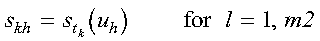
- s
- is the matrix S with elements skh
that contain the interpolation values at (tk,
uh) for k = 1, m1 and
h = 1, m2. Returned as: an lds by (at
least) m2 array, containing numbers of the data type indicated in Table 153.
- The cyclic reduction method used to solve the equations in this subroutine
can generate underflows on well-scaled problems. This does not affect
accuracy, but it may decrease performance. For this reason, you may want to
disable underflow before calling this subroutine.
- Vectors x, y, t, and u, matrix
Z, and the aux work area must have no common elements with
matrix S; otherwise, results are unpredictable.
- The elements within vectors x and y must be
distinct. In addition, the elements in the vectors must be sorted into
ascending order; that is,
x1 < x2 < ...
< xn1 and
y1 < y2 < ...
< yn2. Otherwise, results are
unpredictable. For details on how to do this, see ISORT, SSORT, and DSORT--Sort the Elements of a Sequence.
- You have the option of having the minimum required value for naux
dynamically returned to your program. For details, see "Using Auxiliary Storage in ESSL".
Interpolation is performed at a specified set of
points:
- (tk, uh)
for k = 1, m1 and h = 1,
m2
by fitting bicubic spline functions with natural boundary conditions, using
the following set of data, defined on a rectangular grid,
(xi, yj) for
i = 1, n1 and j = 1,
n2:
- zij for i = 1,
n1 and j = 1, n2
where tk, uh,
xi, yj, and
zij are elements of vectors t,
u, x, and y and matrix Z,
respectively. In vectors x and y, elements are assumed
to be sorted into ascending order.
The interpolation involves two steps:
- For each j from 1 to n2, the single variable cubic
spline:

with natural boundary conditions, is constructed using the data
points:
- (xi, zij)
for i = 1, n1
The following interpolation values are then computed:
- For each k from 1 to m1, the single variable cubic
spline:

with natural boundary conditions, is constructed using the data
points:
The following interpolation values are then computed:
See references [51] and [57]. Because natural boundary
conditions (zero second derivatives at the end of the ranges) are used for the
splines, unless the underlying function has these properties, interpolated
values near the boundaries may be less satisfactory than elsewhere. If
n1, n2, m1, or m2 is 0, no computation is
performed.
Error 2015 is unrecoverable, naux = 0, and unable to
allocate work area.
None
- n1 < 0 or n1 > ldz
- n2 < 0
- m1 < 0 or m1 > lds
- m2 < 0
- ldz < 0
- lds < 0
- Error 2015 is recoverable or naux<>0, and naux is
too small--that is, less than the minimum required value specified in
the syntax for this argument. Return code 1 is returned if error 2015 is
recoverable.
This example computes the interpolated values at a specified set of
points, given by T and U, from a set of data points
defined on a rectangular mesh in the x-y plane, using X,
Y, and Z.
             X   Y   Z   N1  N2 LDZ  T   U   M1  M2  S  LDS  AUX  NAUX
             |   |   |   |   |   |   |   |   |   |   |   |    |    |
CALL SCSIN2( X , Y , Z , 6 , 5 , 6 , T , U , 4 , 3 , S , 4 , AUX , 90 )

X        =  (0.0, 0.2, 0.3, 0.4, 0.5, 0.7)
Y        =  (0.0, 0.2, 0.3, 0.4, 0.6)
        *                                   *
        | 0.000  0.008  0.027  0.064  0.216 |
        | 0.008  0.016  0.035  0.072  0.224 |
Z    =  | 0.027  0.035  0.054  0.091  0.243 |
        | 0.064  0.072  0.091  0.128  0.280 |
        | 0.125  0.133  0.152  0.189  0.341 |
        | 0.343  0.351  0.370  0.407  0.559 |
        *                                   *
T        =  (0.10, 0.15, 0.25, 0.35)
U        =  (0.05, 0.25, 0.45)
        *                     *
        | 0.001  0.017  0.095 |
S    =  | 0.003  0.019  0.097 |
        | 0.016  0.031  0.110 |
        | 0.043  0.059  0.137 |
        *                     *
[ Top of Page | Previous Page | Next Page | Table of Contents | Index ]