This section describes some key points about using the related-computation subroutines.
This section contains the Fourier transform subroutine descriptions.
These subroutines compute a set of m complex discrete
n-point Fourier transforms of complex data.
| X, Y | scale | Subroutine |
| Short-precision complex | Short-precision real | SCFT |
| Long-precision complex | Long-precision real | DCFT |
| Note: | Two invocations of this subroutine are necessary: one to prepare the working storage for the subroutine, and the other to perform the computations. |
| Fortran | CALL SCFT | DCFT (init, x, inc1x, inc2x, y, inc1y, inc2y, n, m, isign, scale, aux1, naux1, aux2, naux2) |
| C and C++ | scft | dcft (init, x, inc1x, inc2x, y, inc1y, inc2y, n, m, isign, scale, aux1, naux1, aux2, naux2); |
| PL/I | CALL SCFT | DCFT (init, x, inc1x, inc2x, y, inc1y, inc2y, n, m, isign, scale, aux1, naux1, aux2, naux2); |
If init <> 0, trigonometric functions and other parameters, depending on arguments other than x, are computed and saved in aux1. The contents of x and y are not used or changed.
If init = 0, the discrete Fourier transforms of the given sequences are computed. The only arguments that may change after initialization are x, y, and aux2. All scalar arguments must be the same as when the subroutine was called for initialization with init <> 0.
Specified as: a fullword integer. It can have any value.
If isign = positive value, Isign = + (transforming time to frequency).
If isign = negative value, Isign = - (transforming frequency to time).
Specified as: a fullword integer; isign > 0 or isign < 0.
If init <> 0, the working storage is computed.
If init = 0, the working storage is used in the computation of the Fourier transforms.
Specified as: an area of storage, containing naux1 long-precision real numbers.
If naux2 = 0 and error 2015 is unrecoverable, aux2 is ignored.
Otherwise, it is the working storage used by this subroutine, which is available for use by the calling program between calls to this subroutine.
Specified as: an area of storage, containing naux2 long-precision real numbers. On output, the contents are overwritten.
If naux2 = 0 and error 2015 is unrecoverable, SCFT and DCFT dynamically allocate the work area used by the subroutine. The work area is deallocated before control is returned to the calling program.
Otherwise, naux2 >= (minimum value required for successful processing). To determine a sufficient value, use the processor-independent formulas. For all other values specified less than the minimum value, you have the option of having the minimum value returned in this argument. For details, see "Using Auxiliary Storage in ESSL".
If init <> 0, this argument is not used, and its contents remain unchanged.
If init = 0, this is array Y, consisting of the results of the m discrete Fourier transforms, each of length n.
Returned as: an array of (at least) length 1+(n-1)inc1y+(m-1)inc2y, containing numbers of the data type indicated in Table 126. This array must be aligned on a doubleword boundary.
If init <> 0, it contains information ready to be passed in a subsequent invocation of this subroutine.
If init = 0, its contents are unchanged.
Returned as: the contents are not relevant.
It is possible to specify sequences in the transposed form--that is, as rows of a two-dimensional array. In this case, inc2x (or inc2y) = 1 and inc1x (or inc1y) is equal to the leading dimension of the array. One can specify either input, output, or both in the transposed form by specifying appropriate values for the stride parameters. For selecting optimal values of inc1x and inc1y for _CFT, you should use STRIDE--Determine the Stride Value for Optimal Performance in Specified Fourier Transform Subroutines. Example 1 in the STRIDE subroutine description explains how it is used for _CFT.
If you specify the same array for X and Y, then inc1x and inc1y must be equal, and inc2x and inc2y must be equal. In this case, output overwrites input. If m = 1, the inc2x and inc2y values are not used by the subroutine. If you specify different arrays for X and Y, they must have no common elements; otherwise, results are unpredictable. See "Concepts".
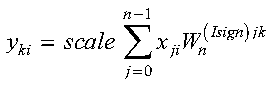
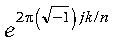
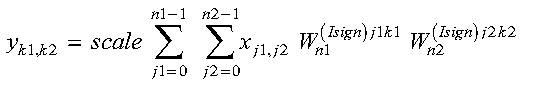
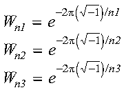
The set of m complex discrete n-point Fourier transforms of complex data in array X, with results going into array Y, is expressed as follows:
for:
where:
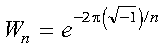
and where:
For scale = 1.0 and isign being positive, you obtain the discrete Fourier transform, a function of frequency. The inverse Fourier transform is obtained with scale = 1.0/n and isign being negative. See references [1], [3], [4], [19], and [20].
Two invocations of this subroutine are necessary:
Error 2015 is unrecoverable, naux2 = 0, and unable to allocate work area.
None
This example shows an input array X with a set of four short-precision complex sequences:
for j = 0, 1, ..., n-1 with n = 8, and the single frequencies k = 0, 1, 2, and 3. The arrays are declared as follows:
     COMPLEX*8  X(0:1023),Y(0:1023)
     REAL*8     AUX1(1693),AUX2(4096)
First, initialize AUX1 using the calling sequence shown below with INIT <> 0. Then use the same calling sequence with INIT = 0 to do the calculation.
          INIT  X INC1X INC2X Y INC1Y INC2Y N   M ISIGN SCALE  AUX1   NAUX1  AUX2   NAUX2
           |    |   |     |   |   |     |   |   |   |     |     |       |     |       |
CALL SCFT(INIT, X , 1  ,  8 , Y , 1  ,  8 , 8 , 4 , 1 , SCALE, AUX1 , 1693 , AUX2 , 4096)
INIT     =  1(for initialization)
INIT     =  0(for computation)
SCALE    =  1.0
X contains the following four sequences:
(1.0000, 0.0000)   (1.0000,  0.0000)   (1.0000,  0.0000)   (1.0000,  0.0000)
(1.0000, 0.0000)   (0.7071,  0.7071)   (0.0000,  1.0000)  (-0.7071,  0.7071)
(1.0000, 0.0000)   (0.0000,  1.0000)  (-1.0000,  0.0000)   (0.0000, -1.0000)
(1.0000, 0.0000)  (-0.7071,  0.7071)   (0.0000, -1.0000)   (0.7071,  0.7071)
(1.0000, 0.0000)  (-1.0000,  0.0000)   (1.0000,  0.0000)  (-1.0000,  0.0000)
(1.0000, 0.0000)  (-0.7071, -0.7071)   (0.0000,  1.0000)   (0.7071, -0.7071)
(1.0000, 0.0000)   (0.0000, -1.0000)  (-1.0000,  0.0000)   (0.0000,  1.0000)
(1.0000, 0.0000)   (0.7071, -0.7071)   (0.0000, -1.0000)  (-0.7071, -0.7071)
Y contains the following four sequences:
(8.0000, 0.0000)  (0.0000, 0.0000)  (0.0000, 0.0000)  (0.0000, 0.0000)
(0.0000, 0.0000)  (8.0000, 0.0000)  (0.0000, 0.0000)  (0.0000, 0.0000)
(0.0000, 0.0000)  (0.0000, 0.0000)  (8.0000, 0.0000)  (0.0000, 0.0000)
(0.0000, 0.0000)  (0.0000, 0.0000)  (0.0000, 0.0000)  (8.0000, 0.0000)
(0.0000, 0.0000)  (0.0000, 0.0000)  (0.0000, 0.0000)  (0.0000, 0.0000)
(0.0000, 0.0000)  (0.0000, 0.0000)  (0.0000, 0.0000)  (0.0000, 0.0000)
(0.0000, 0.0000)  (0.0000, 0.0000)  (0.0000, 0.0000)  (0.0000, 0.0000)
(0.0000, 0.0000)  (0.0000, 0.0000)  (0.0000, 0.0000)  (0.0000, 0.0000)
This example shows an input array X with a set of four input spike sequences equal to the output of Example 1. This shows how you can compute the inverse of the transform in Example 1 by using a negative isign, giving as output the four sequences listed in the input for Example 1. First, initialize AUX1 using the calling sequence shown below with INIT <> 0. Then use the same calling sequence with INIT = 0 to do the calculation.
          INIT  X INC1X INC2X Y INC1Y INC2Y N   M  ISIGN SCALE   AUX1   NAUX1  AUX2   NAUX2
           |    |   |     |   |   |     |   |   |    |     |      |       |     |       |
CALL SCFT(INIT, X , 1  ,  8 , Y , 1  ,  8 , 8 , 4 , -1 , SCALE , AUX1 , 1693 , AUX2 , 4096)
INIT     =  1(for initialization)
INIT     =  0(for computation)
SCALE    =  0.125
X        =(same as output Y in Example 1)
Y =(same as input X in Example 1)
This example shows an input array X with a set of four short-precision complex sequences
for j = 0, 1, ..., n-1 with n = 12, and the single frequencies k = 0, 1, 2, and 3. Also, inc1x = inc1y = m and inc2x = inc2y = 1 to show how the input and output arrays can be stored in the transposed form. The arrays are declared as follows:
     COMPLEX*8  X (4,0:11),Y(4,0:11)
     REAL*8     AUX1(10000),AUX2(10000)
First, initialize AUX1 using the calling sequence shown below with INIT <> 0. Then use the same calling sequence with INIT = 0 to do the calculation.
          INIT  X INC1X INC2X Y INC1Y INC2Y  N   M ISIGN SCALE  AUX1   NAUX1   AUX2   NAUX2
           |    |   |     |   |   |     |    |   |   |     |     |       |      |       |
CALL SCFT(INIT, X , 4  ,  1 , Y , 4  ,  1 , 12 , 4 , 1 , SCALE, AUX1 , 10000 , AUX2 , 10000)
INIT     =  1(for initialization)
INIT     =  0(for computation)
SCALE    =  1.0
X contains the following four sequences:
(1.0000, 0.0000)   (1.0000, 0.0000)   (1.0000, 0.0000)   (1.0000, 0.0000)
(1.0000, 0.0000)   (0.8660, 0.5000)   (0.5000, 0.8660)   (0.0000, 1.0000)
(1.0000, 0.0000)   (0.5000, 0.8660)  (-0.5000, 0.8660)  (-1.0000, 0.0000)
(1.0000, 0.0000)   (0.0000, 1.0000)  (-1.0000, 0.0000)  (0.0000, -1.0000)
(1.0000, 0.0000)  (-0.5000, 0.8660) (-0.5000, -0.8660)   (1.0000, 0.0000)
(1.0000, 0.0000)  (-0.8660, 0.5000)  (0.5000, -0.8660)   (0.0000, 1.0000)
(1.0000, 0.0000)  (-1.0000, 0.0000)   (1.0000, 0.0000)  (-1.0000, 0.0000)
(1.0000, 0.0000) (-0.8660, -0.5000)   (0.5000, 0.8660)  (0.0000, -1.0000)
(1.0000, 0.0000) (-0.5000, -0.8660)  (-0.5000, 0.8660)   (1.0000, 0.0000)
(1.0000, 0.0000)  (0.0000, -1.0000)  (-1.0000, 0.0000)   (0.0000, 1.0000)
(1.0000, 0.0000)  (0.5000, -0.8660) (-0.5000, -0.8660) (-1.0000,  0.0000)
(1.0000, 0.0000)  (0.8660, -0.5000)  (0.5000, -0.8660)  (0.0000, -1.0000)
Y contains the following four sequences:
(12.0000, 0.0000)   (0.0000, 0.0000)   (0.0000, 0.0000)   (0.0000, 0.0000)
 (0.0000, 0.0000)  (12.0000, 0.0000)   (0.0000, 0.0000)   (0.0000, 0.0000)
 (0.0000, 0.0000)   (0.0000, 0.0000)  (12.0000, 0.0000)   (0.0000, 0.0000)
 (0.0000, 0.0000)   (0.0000, 0.0000)   (0.0000, 0.0000)  (12.0000, 0.0000)
 (0.0000, 0.0000)   (0.0000, 0.0000)   (0.0000, 0.0000)   (0.0000, 0.0000)
 (0.0000, 0.0000)   (0.0000, 0.0000)   (0.0000, 0.0000)   (0.0000, 0.0000)
 (0.0000, 0.0000)   (0.0000, 0.0000)   (0.0000, 0.0000)   (0.0000, 0.0000)
 (0.0000, 0.0000)   (0.0000, 0.0000)   (0.0000, 0.0000)   (0.0000, 0.0000)
 (0.0000, 0.0000)   (0.0000, 0.0000)   (0.0000, 0.0000)   (0.0000, 0.0000)
 (0.0000, 0.0000)   (0.0000, 0.0000)   (0.0000, 0.0000)   (0.0000, 0.0000)
 (0.0000, 0.0000)   (0.0000, 0.0000)   (0.0000, 0.0000)   (0.0000, 0.0000)
 (0.0000, 0.0000)   (0.0000, 0.0000)   (0.0000, 0.0000)   (0.0000, 0.0000)
This example shows an input array X with a set of four input spike sequences exactly equal to the output of Example 3. This shows how you can compute the inverse of the transform in Example 3 by using a negative isign, giving as output the four sequences listed in the input for Example 3. First, initialize AUX1 using the calling sequence shown below with INIT <> 0. Then use the same calling sequence with INIT = 0 to do the calculation.
          INIT  X INC1X INC2X Y INC1Y INC2Y  N   M  ISIGN SCALE   AUX1  NAUX1  AUX2  NAUX2
           |    |   |     |   |   |     |    |   |    |     |      |      |     |      |
CALL SCFT(INIT, X , 4  ,  1 , Y , 4  ,  1 , 12 , 4 , -1 , SCALE , AUX1, 10000, AUX2, 10000)
INIT     =  1(for initialization)
INIT     =  0(for computation)
SCALE    =  1.0/12.0
X        =(same as output Y in Example 3)
Y =(same as input X in Example 3)
This example shows how to compute a transform of a single long-precision complex sequence. It uses isign = 1 and scale = 1.0. The arrays are declared as follows:
     COMPLEX*16  X(0:7),Y(0:7)
     REAL*8      AUX1(26),AUX2(12)
The input in X is an impulse at zero, and the output in Y is constant for all frequencies. First, initialize AUX1 using the calling sequence shown below with INIT <> 0. Then use the same calling sequence with INIT = 0 to do the calculation.
          INIT  X INC1X INC2X Y INC1Y INC2Y N   M ISIGN SCALE   AUX1  NAUX1  AUX2  NAUX2
           |    |   |     |   |   |     |   |   |   |     |      |      |     |      |
CALL DCFT(INIT, X , 1  ,  0 , Y , 1  ,  0 , 8 , 1 , 1 , SCALE , AUX1 , 26  , AUX2 , 12)
INIT     =  1(for initialization)
INIT     =  0(for computation)
SCALE    =  1.0
X contains the following sequence:
(1.0000, 0.0000)
(0.0000, 0.0000)
(0.0000, 0.0000)
(0.0000, 0.0000)
(0.0000, 0.0000)
(0.0000, 0.0000)
(0.0000, 0.0000)
(0.0000, 0.0000)
(1.0000, 0.0000)
(1.0000, 0.0000)
(1.0000, 0.0000)
(1.0000, 0.0000)
(1.0000, 0.0000)
(1.0000, 0.0000)
(1.0000, 0.0000)
(1.0000, 0.0000)
These subroutines compute a set of m complex discrete
n-point Fourier transforms of real data.
| X, scale | Y | Subroutine |
| Short-precision real | Short-precision complex | SRCFT |
| Long-precision real | Long-precision complex | DRCFT |
| Note: | Two invocations of this subroutine are necessary: one to prepare the working storage for the subroutine, and the other to perform the computations. |
| Fortran | CALL SRCFT (init, x, inc2x, y,
inc2y, n, m, isign, scale,
aux1, naux1, aux2, naux2, aux3,
naux3)
CALL DRCFT (init, x, inc2x, y, inc2y, n, m, isign, scale, aux1, naux1, aux2, naux2) |
| C and C++ | srcft (init, x, inc2x, y,
inc2y, n, m, isign, scale,
aux1, naux1, aux2, naux2, aux3,
naux3);
drcft (init, x, inc2x, y, inc2y, n, m, isign, scale, aux1, naux1, aux2, naux2); |
| PL/I | CALL SRCFT (init, x, inc2x, y,
inc2y, n, m, isign, scale,
aux1, naux1, aux2, naux2, aux3,
naux3);
CALL DRCFT (init, x, inc2x, y, inc2y, n, m, isign, scale, aux1, naux1, aux2, naux2); |
If init <> 0, trigonometric functions and other parameters, depending on arguments other than x, are computed and saved in aux1. The contents of x and y are not used or changed.
If init = 0, the discrete Fourier transforms of the given sequences are computed. The only arguments that may change after initialization are x, y, and aux2. All scalar arguments must be the same as when the subroutine was called for initialization with init <> 0.
Specified as: a fullword integer. It can have any value.
If isign = positive value, Isign = + (transforming time to frequency).
If isign = negative value, Isign = - (transforming frequency to time).
Specified as: a fullword integer; isign > 0 or isign < 0.
If init <> 0, the working storage is computed.
If init = 0, the working storage is used in the computation of the Fourier transforms.
Specified as: an area of storage, containing naux1 long-precision real numbers.
If naux2 = 0 and error 2015 is unrecoverable, aux2 is ignored.
Otherwise, it is the working storage used by this subroutine, which is available for use by the calling program between calls to this subroutine.
Specified as: an area of storage, containing naux2 long-precision real numbers. On output, the contents are overwritten.
If naux2 = 0 and error 2015 is unrecoverable, SRCFT and DRCFT dynamically allocate the work area used by the subroutine. The work area is deallocated before control is returned to the calling program.
Otherwise, naux2 >= (minimum value required for successful processing). To determine a sufficient value, use the processor-independent formulas. For all other values specified less than the minimum value, you have the option of having the minimum value returned in this argument. For details, see "Using Auxiliary Storage in ESSL".
Specified as: an area of storage, containing naux3 long-precision real numbers.
Specified as: a fullword integer.
If init <> 0, this argument is not used, and its contents remain unchanged.
If init = 0, this is array Y, consisting of the results of the m complex discrete Fourier transforms, each of length n. The sequences are stored with the stride 1. Due to complex conjugate symmetry, only the first (n/2) + 1 elements of each sequence are given in the output--that is, yki, k = 0, 1, ..., n/2, i = 1, 2, ..., m.
Returned as: an array of (at least) length n/2+1+(m-1)inc2y, containing numbers of the data type indicated in Table 127. This array must be aligned on a doubleword boundary. (It can be declared as Y(inc2y,m).)
If init <> 0, it contains information ready to be passed in a subsequent invocation of this subroutine.
If init = 0, its contents are unchanged.
Returned as: the contents are not relevant.
If you specify the same array for X and Y, then inc2x must equal 2(inc2y). In this case, output overwrites input. If m = 1, the inc2x and inc2y values are not used by the subroutine. If you specify different arrays for X and Y, they must have no common elements; otherwise, results are unpredictable. See "Concepts".
The set of m complex conjugate even discrete n-point Fourier transforms of real data in array X, with results going into array Y, is expressed as follows:
for:
where:
and where:
The output in array Y is complex. For scale = 1.0 and isign being positive, you obtain the discrete Fourier transform, a function of frequency. The inverse Fourier transform is obtained with scale = 1.0/n and isign being negative. See references [1], [4], [19], and [20].
Two invocations of this subroutine are necessary:
Error 2015 is unrecoverable, naux2 = 0, and unable to allocate work area.
None
This example shows an input array X with a set of m cosine sequences cos(2pijk/n), j = 0, 1, ..., 15 with the single frequencies k = 0, 1, 2, 3. The Fourier transform of the cosine sequence with frequency k = 0 or n/2 has 1.0 in the 0 or n/2 position, respectively, and zeros elsewhere. For all other k, the Fourier transform has 0.5 in the k position and zeros elsewhere. The arrays are declared as follows:
     REAL*4     X(0:65535)
     COMPLEX*8  Y(0:32768)
     REAL*8     AUX1(41928), AUX2(35344), AUX3(1)
First, initialize AUX1 using the calling sequence shown below with INIT <> 0. Then use the same calling sequence with INIT = 0 to do the calculation.
           INIT  X  INC2X Y INC2Y  N   M ISIGN SCALE  AUX1   NAUX1   AUX2   NAUX2   AUX3  NAUX3
            |    |    |   |   |    |   |   |     |     |       |      |       |      |      |
CALL SRCFT(INIT, X , 16 , Y , 9 , 16 , 4 , 1 , SCALE, AUX1 , 41928 , AUX2 , 35344 , AUX3 ,  0 )
INIT     =  1(for initialization)
INIT     =  0(for computation)
SCALE    =  1.0/16
X contains the following four sequences:
1.0000   1.0000   1.0000   1.0000
1.0000   0.9239   0.7071   0.3827
1.0000   0.7071   0.0000  -0.7071
1.0000   0.3827  -0.7071  -0.9239
1.0000   0.0000  -1.0000   0.0000
1.0000  -0.3827  -0.7071   0.9239
1.0000  -0.7071   0.0000   0.7071
1.0000  -0.9239   0.7071  -0.3827
1.0000  -1.0000   1.0000  -1.0000
1.0000  -0.9239   0.7071  -0.3827
1.0000  -0.7071   0.0000   0.7071
1.0000  -0.3827  -0.7071   0.9239
1.0000   0.0000  -1.0000   0.0000
1.0000   0.3827  -0.7071  -0.9239
1.0000   0.7071   0.0000  -0.7071
1.0000   0.9239   0.7071   0.3827
Y contains the following four sequences:
(1.0000, 0.0000)  (0.0000, 0.0000)  (0.0000, 0.0000)  (0.0000, 0.0000)
(0.0000, 0.0000)  (0.5000, 0.0000)  (0.0000, 0.0000)  (0.0000, 0.0000)
(0.0000, 0.0000)  (0.0000, 0.0000)  (0.5000, 0.0000)  (0.0000, 0.0000)
(0.0000, 0.0000)  (0.0000, 0.0000)  (0.0000, 0.0000)  (0.5000, 0.0000)
(0.0000, 0.0000)  (0.0000, 0.0000)  (0.0000, 0.0000)  (0.0000, 0.0000)
(0.0000, 0.0000)  (0.0000, 0.0000)  (0.0000, 0.0000)  (0.0000, 0.0000)
(0.0000, 0.0000)  (0.0000, 0.0000)  (0.0000, 0.0000)  (0.0000, 0.0000)
(0.0000, 0.0000)  (0.0000, 0.0000)  (0.0000, 0.0000)  (0.0000, 0.0000)
(0.0000, 0.0000)  (0.0000, 0.0000)  (0.0000, 0.0000)  (0.0000, 0.0000)
This example shows another transform computation with different data using the same initialized array AUX1 as in Example 1. The input is also a set of four cosine sequences cos(2pijk/n), j = 0, 1, ..., 15 with the single frequencies k = 8, 9, 10, 11, thus including the middle frequency k = 8. The middle frequency has the value 1.0. For other frequencies, the transform has zeros, except for frequencies k and n-k. Only the values for j = n-k are given in the output.
           INIT X  INC2X Y INC2Y  N   M ISIGN SCALE  AUX1   NAUX1   AUX2   NAUX2   AUX3  NAUX3
            |   |    |   |   |    |   |   |     |     |       |      |       |      |
CALL SRCFT( 0 , X , 16 , Y , 9 , 16 , 4 , 1 , SCALE, AUX1 , 41928 , AUX2 , 35344 , AUX3 ,  0  )
SCALE = 1.0/16
X contains the following four sequences:
 1.0000   1.0000   1.0000   1.0000
-1.0000  -0.9239  -0.7071  -0.3827
 1.0000   0.7071   0.0000  -0.7071
-1.0000  -0.3827   0.7071   0.9239
 1.0000   0.0000  -1.0000   0.0000
-1.0000   0.3827   0.7071  -0.9239
 1.0000  -0.7071   0.0000   0.7071
-1.0000   0.9239  -0.7071   0.3827
 1.0000  -1.0000   1.0000  -1.0000
-1.0000   0.9239  -0.7071   0.3827
 1.0000  -0.7071   0.0000   0.7071
-1.0000   0.3827   0.7071  -0.9239
 1.0000   0.0000  -1.0000   0.0000
-1.0000  -0.3827   0.7071   0.9239
 1.0000   0.7071   0.0000  -0.7071
-1.0000  -0.9239  -0.7071  -0.3827
Y contains the following four sequences:
(0.0000, 0.0000)  (0.0000, 0.0000)  (0.0000, 0.0000)  (0.0000, 0.0000)
(0.0000, 0.0000)  (0.0000, 0.0000)  (0.0000, 0.0000)  (0.0000, 0.0000)
(0.0000, 0.0000)  (0.0000, 0.0000)  (0.0000, 0.0000)  (0.0000, 0.0000)
(0.0000, 0.0000)  (0.0000, 0.0000)  (0.0000, 0.0000)  (0.0000, 0.0000)
(0.0000, 0.0000)  (0.0000, 0.0000)  (0.0000, 0.0000)  (0.0000, 0.0000)
(0.0000, 0.0000)  (0.0000, 0.0000)  (0.0000, 0.0000)  (0.5000, 0.0000)
(0.0000, 0.0000)  (0.0000, 0.0000)  (0.5000, 0.0000)  (0.0000, 0.0000)
(0.0000, 0.0000)  (0.5000, 0.0000)  (0.0000, 0.0000)  (0.0000, 0.0000)
(1.0000, 0.0000)  (0.0000, 0.0000)  (0.0000, 0.0000)  (0.0000, 0.0000)
This example uses the mixed-radix capability. The arrays are declared as follows:
     REAL*8     X(0:11)
     COMPLEX*16 Y(0:6)
     REAL*8     AUX1(50),AUX2(50)
Arrays X and Y are made equivalent by the following statement, making them occupy the same storage:
EQUIVALENCE (X,Y)
First, initialize AUX1 using the calling sequence shown below with INIT <> 0. Then use the same calling sequence with INIT = 0 to do the calculation.
           INIT  X INC2X Y INC2Y  N   M ISIGN SCALE   AUX1  NAUX1 AUX2  NAUX2
            |    |   |   |   |    |   |   |     |      |      |    |      |
CALL DRCFT(INIT, X , 0 , Y , 0 , 12 , 1 , 1 , SCALE , AUX1 , 50 , AUX2 , 50)
INIT     =  1(for initialization)
INIT     =  0(for computation)
SCALE    =  1.0
X        =  (1.0000 , 1.0000 , 1.0000 , 1.0000 , 1.0000 , 1.0000 ,
             1.0000 , 1.0000 , 1.0000 , 1.0000 , 1.0000 , 1.0000)
Y contains the following sequence:
(12.0000 , 0.0000)
 (0.0000 , 0.0000)
 (0.0000 , 0.0000)
 (0.0000 , 0.0000)
 (0.0000 , 0.0000)
 (0.0000 , 0.0000)
 (0.0000 , 0.0000)
These subroutines compute a set of m real discrete
n-point Fourier transforms of complex conjugate even data.
| X | Y, scale | Subroutine |
| Short-precision complex | Short-precision real | SCRFT |
| Long-precision complex | Long-precision real | DCRFT |
| Note: | Two invocations of this subroutine are necessary: one to prepare the working storage for the subroutine, and the other to perform the computations. |
| Fortran | CALL SCRFT (init, x, inc2x, y,
inc2y, n, m, isign, scale,
aux1, naux1, aux2, naux2, aux3,
naux3)
CALL DCRFT (init, x, inc2x, y, inc2y, n, m, isign, scale, aux1, naux1, aux2, naux2) |
| C and C++ | scrft (init, x, inc2x, y,
inc2y, n, m, isign, scale,
aux1, naux1, aux2, naux2, aux3,
naux3);
dcrft (init, x, inc2x, y, inc2y, n, m, isign, scale, aux1, naux1, aux2, naux2); |
| PL/I | CALL SCRFT (init, x, inc2x, y,
inc2y, n, m, isign, scale,
aux1, naux1, aux2, naux2, aux3,
naux3);
CALL DCRFT (init, x, inc2x, y, inc2y, n, m, isign, scale, aux1, naux1, aux2, naux2); |
If init <> 0, trigonometric functions and other parameters, depending on arguments other than x, are computed and saved in aux1. The contents of x and y are not used or changed.
If init = 0, the discrete Fourier transforms of the given sequences are computed. The only arguments that may change after initialization are x, y, and aux2. All scalar arguments must be the same as when the subroutine was called for initialization with init <> 0.
Specified as: a fullword integer. It can have any value.
Specified as: an array of (at least) length n/2+1+(m-1)inc2x, containing numbers of the data type indicated in Table 128. This array must be aligned on a doubleword boundary. (It can be declared as X(inc2x,m).)
If isign = positive value, Isign = + (transforming time to frequency).
If isign = negative value, Isign = - (transforming frequency to time).
Specified as: a fullword integer; isign > 0 or isign < 0.
If init <> 0, the working storage is computed.
If init = 0, the working storage is used in the computation of the Fourier transforms.
Specified as: an area of storage, containing naux1 long-precision real numbers.
If naux2 = 0 and error 2015 is unrecoverable, aux2 is ignored.
Otherwise, it is the working storage used by this subroutine that is available for use by the calling program between calls to this subroutine.
Specified as: an area of storage, containing naux2 long-precision real numbers. On output, the contents are overwritten.
If naux2 = 0 and error 2015 is unrecoverable, SCRFT and DCRFT dynamically allocate the work area used by the subroutine. The work area is deallocated before control is returned to the calling program.
Otherwise, naux2 >= (minimum value required for successful processing). To determine a sufficient value, use the processor-independent formulas. For all other values specified less than the minimum value, you have the option of having the minimum value returned in this argument. For details, see "Using Auxiliary Storage in ESSL".
Specified as: an area of storage, containing naux3 long-precision real numbers.
Specified as: a fullword integer.
If init <> 0, this argument is not used, and its contents remain unchanged.
If init = 0, this is array Y, consisting of the results of the m discrete Fourier transforms of the complex conjugate even data, each of length n. The sequences are stored with stride 1.
Returned as: an array of (at least) length n+(m-1)inc2y, containing numbers of the data type indicated in Table 128. See "Notes" for more details. (It can be declared as Y(inc2y,m).)
If init <> 0, it contains information ready to be passed in a subsequent invocation of this subroutine.
If init = 0, its contents are unchanged.
Returned as: the contents are not relevant.
If you specify the same array for X and Y, then inc2y must equal 2(inc2x). In this case, output overwrites input. If m = 1, the inc2x and inc2y values are not used by the subroutine. If you specify different arrays for X and Y, they must have no common elements; otherwise, results are unpredictable. See "Concepts".
The set of m real discrete n-point Fourier transforms of complex conjugate even data in array X, with results going into array Y, is expressed as follows:
for:
where:
and where:
Because of the symmetry, Y has real data. For scale = 1.0 and isign being positive, you obtain the discrete Fourier transform, a function of frequency. The inverse Fourier transform is obtained with scale = 1.0/n and isign being negative. See references [1], [4], [19], and [20].
Two invocations of this subroutine are necessary:
Error 2015 is unrecoverable, naux2 = 0, and unable to allocate work area.
None
This example uses the mixed-radix capability and shows how to compute a single transform. The arrays are declared as follows:
     COMPLEX*8  X(0:6)
     REAL*8     AUX1(50), AUX2(50), AUX3(1)
     REAL*4     Y(0:11)
First, initialize AUX1 using the calling sequence shown below with INIT <> 0. Then use the same calling sequence with INIT = 0 to do the calculation.
| Note: | X shows the n/2+1 = 7 elements used in the computation. |
           INIT  X INC2X Y INC2Y  N   M ISIGN SCALE  AUX1  NAUX1 AUX2  NAUX2  AUX3  NAUX3
            |    |   |   |   |    |   |   |     |     |      |     |     |     |      |
CALL SCRFT(INIT, X , 0 , Y , 0 , 12 , 1 , 1 , SCALE, AUX1 , 50 , AUX2 , 50 ,  AUX3 ,  0  )
INIT     =  1(for initialization)
INIT     =  0(for computation)
SCALE    =  1.0
X contains the following sequence:
(1.0,  0.0)
(0.0,  0.0)
(0.0,  0.0)
(0.0,  0.0)
(0.0,  0.0)
(0.0,  0.0)
(0.0,  0.0)
Y = (1.0, 1.0, 1.0, 1.0, 1.0, 1.0, 1.0, 1.0, 1.0, 1.0, 1.0, 1.0)
This example shows another transform computation with different data using the same initialized array AUX1 as in Example 1.
          INIT  X INC2X Y INC2Y  N   M ISIGN SCALE  AUX1 NAUX1  AUX2 NAUX2  AUX3  NAUX3
           |    |   |   |   |    |   |   |     |     |     |     |     |     |      |
CALL SCRFT( 0 , X , 0 , Y , 0 , 12 , 1 , 1 , SCALE, AUX1 , 50 , AUX2 , 50 , AUX3 ,  0 )
SCALE = 1.0
X contains the following sequence:
(1.0, 0.0)
(1.0, 0.0)
(1.0, 0.0)
(1.0, 0.0)
(1.0, 0.0)
(1.0, 0.0)
(1.0, 0.0)
Y        =  (12.0 , 0.0 , 0.0 , 0.0 , 0.0 , 0.0 , 0.0 , 0.0 ,
             0.0 , 0.0 , 0.0 , 0.0)
This example shows how to compute many transforms simultaneously. The arrays are declared as follows:
     COMPLEX*8  X(0:8,2)
     REAL*8     AUX1(50), AUX2(16), AUX3(1)
     REAL*4     Y(0:15,2)
First, initialize AUX1 using the calling sequence shown below with INIT <> 0. Then use the same calling sequence with INIT = 0 to do the calculation.
           INIT  X INC2X Y INC2Y   N   M ISIGN SCALE  AUX1  NAUX1 AUX2  NAUX2 AUX3  NAUX3
            |    |   |   |   |     |   |   |     |     |      |    |      |    |      |
CALL SCRFT(INIT, X , 9 , Y , 16 , 16 , 2 , 1 , SCALE, AUX1 , 50 , AUX2 , 16 , AUX3 ,  0 )
INIT     =  1(for initialization)
INIT     =  0(for computation)
SCALE    =  1.0
X contains the following two sequences:
(1.0, 0.0)  (0.0, 0.0)
(1.0, 0.0)  (0.0, 0.0)
(1.0, 0.0)  (0.0, 0.0)
(1.0, 0.0)  (0.0, 0.0)
(1.0, 0.0)  (0.0, 0.0)
(1.0, 0.0)  (0.0, 0.0)
(1.0, 0.0)  (0.0, 0.0)
(1.0, 0.0)  (0.0, 0.0)
(1.0, 0.0)  (1.0, 0.0)
Y contains the following two sequences:
16.0   1.0
 0.0  -1.0
 0.0   1.0
 0.0  -1.0
 0.0   1.0
 0.0  -1.0
 0.0   1.0
 0.0  -1.0
 0.0   1.0
 0.0  -1.0
 0.0   1.0
 0.0  -1.0
 0.0   1.0
 0.0  -1.0
 0.0   1.0
 0.0  -1.0
This example shows the same array being used for input and output. The arrays are declared as follows:
     COMPLEX*16 X(0:8,2)
     REAL*8     AUX1(50), AUX2(16)
     REAL*8     Y(0:17,2)
Arrays X and Y are made equivalent by the following statement, making them occupy the same storage:
EQUIVALENCE (X,Y)
This requires INC2Y = 2(INC2X). First, initialize AUX1 using the calling sequence shown below with INIT <> 0. Then use the same calling sequence with INIT = 0 to do the calculation.
           INIT  X INC2X Y  INC2Y  N   M  ISIGN SCALE  AUX1  NAUX1 AUX2  NAUX2
            |    |   |   |    |    |   |    |     |     |      |    |      |
CALL DCRFT(INIT, X , 9 , Y , 18 , 16 , 2 , -1 , SCALE, AUX1 , 50 , AUX2 , 16)
INIT     =  1(for initialization)
INIT     =  0(for computation)
SCALE    =  0.0625
X contains the following two sequences:
 (1.0,  0.0)   (1.0,  0.0)
 (0.0,  1.0)   (0.0, -1.0)
(-1.0,  0.0)  (-1.0,  0.0)
 (0.0, -1.0)   (0.0,  1.0)
 (1.0,  0.0)   (1.0,  0.0)
 (0.0,  1.0)   (0.0, -1.0)
(-1.0,  0.0)  (-1.0,  0.0)
 (0.0, -1.0)   (0.0,  1.0)
 (1.0,  0.0)   (1.0,0.0)
Y contains the following two sequences:
0.0  0.0
0.0  0.0
0.0  0.0
0.0  0.0
0.0  1.0
0.0  0.0
0.0  0.0
0.0  0.0
0.0  0.0
0.0  0.0
0.0  0.0
0.0  0.0
1.0  0.0
0.0  0.0
0.0  0.0
0.0  0.0
These subroutines compute a set of m real even discrete n-point Fourier transforms of cosine sequences of real even data.
| X, Y, scale | Subroutine |
| Short-precision real | SCOSF |
| Long-precision real | DCOSF |
| Note: | Two invocations of this subroutine are necessary: one to prepare the working storage for the subroutine, and the other to perform the computations. |
| Fortran | CALL SCOSF | DCOSF (init, x, inc1x, inc2x, y, inc1y, inc2y, n, m, scale, aux1, naux1, aux2, naux2) |
| C and C++ | scosf | dcosf (init, x, inc1x, inc2x, y, inc1y, inc2y, n, m, scale, aux1, naux1, aux2, naux2); |
| PL/I | CALL SCOSF | DCOSF (init, x, inc1x, inc2x, y, inc1y, inc2y, n, m, scale, aux1, naux1, aux2, naux2); |
If init <> 0, trigonometric functions and other parameters, depending on arguments other than x, are computed and saved in aux1. The contents of x and y are not used or changed.
If init = 0, the discrete Fourier transforms of the given sequences are computed. The only arguments that may change after initialization are x, y, and aux2. All scalar arguments must be the same as when the subroutine was called for initialization with init <> 0.
Specified as: a fullword integer. It can have any value.
If init <> 0, the working storage is computed.
If init = 0, the working storage is used in the computation of the Fourier transforms.
Specified as: an area of storage, containing naux1 long-precision real numbers.
If naux2 = 0 and error 2015 is unrecoverable, aux2 is ignored.
Otherwise, it is the working storage used by this subroutine, which is available for use by the calling program between calls to this subroutine.
Specified as: an area of storage, containing naux2 long-precision real numbers. On output, the contents are overwritten.
If naux2 = 0 and error 2015 is unrecoverable, SCOSF and DCOSF dynamically allocate the work area used by the subroutine. The work area is deallocated before control is returned to the calling program.
Otherwise, naux2 >= (minimum value required for successful processing). To determine a sufficient value, use the processor-independent formulas. For all other values specified less than the minimum value, you have the option of having the minimum value returned in this argument. For details, see "Using Auxiliary Storage in ESSL".
If init <> 0, this argument is not used, and its contents remain unchanged.
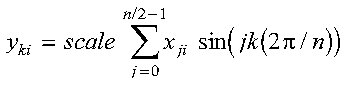
If init = 0, this is array Y, consisting of the results of the m discrete Fourier transforms, where each Fourier transform is real and of length n. However, due to symmetry, only the first n/2+1 values are given in the output--that is, yki, k = 0, 1, ..., n/2 for each i = 1, 2, ..., m.
Returned as: an array of (at least) length 1+(n/2)inc1y+(m-1)inc2y, containing numbers of the data type indicated in Table 129.
If init <> 0, it contains information ready to be passed in a subsequent invocation of this subroutine.
If init = 0, its contents are unchanged.
Returned as: the contents are not relevant.
It is possible to specify sequences in the transposed form--that is, as rows of a two-dimensional array. In this case, inc2x (or inc2y) = 1 and inc1x (or inc1y) is equal to the leading dimension of the array. One can specify either input, output, or both in the transposed form by specifying appropriate values for the stride parameters. For selecting optimal values of inc1x and inc1y for _COSF, you should use STRIDE--Determine the Stride Value for Optimal Performance in Specified Fourier Transform Subroutines. Example 2 in the STRIDE subroutine description explains how it is used for _COSF.
If you specify the same array for X and Y, then inc1x and inc1y must be equal, and inc2x and inc2y must be equal. In this case, output overwrites input. If m = 1, the inc2x and inc2y values are not used by the subroutine. If you specify different arrays for X and Y, they must have no common elements; otherwise, results are unpredictable. See "Concepts".
The set of m real even discrete n-point Fourier transforms of the cosine sequences of real data in array X, with results going into array Y, is expressed as follows:
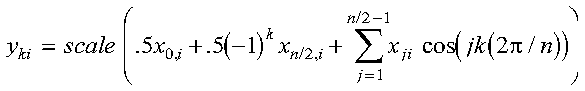
for:
where:
You can obtain the inverse cosine transform by specifying scale = 4.0/n. Thus, if an X input is used with scale = 1.0, and its output is used as input on a subsequent call with scale = 4.0/n, the original X is obtained. See references [1], [4], [19], and [20].
Two invocations of this subroutine are necessary:
These subroutines use a Fourier transform method with a mixed-radix capability. This provides maximum performance for your application.
Error 2015 is unrecoverable, naux2 = 0, and unable to allocate work area.
None
This example shows an input array X with a set of m cosine sequences of length n/2+1, cos(jk(2pi/n)), j = 0, 1, ..., n/2, with the single frequencies k = 0, 1, 2, 3. The Fourier transform of the cosine sequence with frequency k = 0 or n/2 has n/2 in the 0-th or n/2-th position, respectively, and zeros elsewhere. For all other k, the Fourier transform has n/4 in position k and zeros elsewhere. The arrays are declared as follows:
     REAL*4     X(0:71),Y(0:71)
     REAL*8     AUX1(414),AUX2(8960)
First, initialize AUX1 using the calling sequence shown below with INIT <> 0. Then use the same calling sequence with INIT = 0 to do the calculation.
           INIT  X INC1X INC2X Y INC1Y INC2Y  N   M   SCALE  AUX1  NAUX1  AUX2  NAUX2
            |    |   |     |   |   |     |    |   |    |      |      |     |      |
CALL SCOSF(INIT, X , 1  , 18 , Y , 1  , 18 , 32 , 4 , SCALE, AUX1 , 414 , AUX2 , 8960)
INIT     =  1(for initialization)
INIT     =  0(for computation)
SCALE    =  1.0
X contains the following four sequences:
1.0000   1.0000   1.0000   1.0000
1.0000   0.9808   0.9239   0.8315
1.0000   0.9239   0.7071   0.3827
1.0000   0.8315   0.3827  -0.1951
1.0000   0.7071   0.0000  -0.7071
1.0000   0.5556  -0.3827  -0.9808
1.0000   0.3827  -0.7071  -0.9239
1.0000   0.1951  -0.9239  -0.5556
1.0000   0.0000  -1.0000   0.0000
1.0000  -0.1951  -0.9239   0.5556
1.0000  -0.3827  -0.7071   0.9239
1.0000  -0.5556  -0.3827   0.9808
1.0000  -0.7071   0.0000   0.7071
1.0000  -0.8315   0.3827   0.1951
1.0000  -0.9239   0.7071  -0.3827
1.0000  -0.9808   0.9239  -0.8315
1.0000  -1.0000   1.0000  -1.0000
 .        .        .        .
Y contains the following four sequences:
16.0000  0.0000  0.0000  0.0000
 0.0000  8.0000  0.0000  0.0000
 0.0000  0.0000  8.0000  0.0000
 0.0000  0.0000  0.0000  8.0000
 0.0000  0.0000  0.0000  0.0000
 0.0000  0.0000  0.0000  0.0000
 0.0000  0.0000  0.0000  0.0000
 0.0000  0.0000  0.0000  0.0000
 0.0000  0.0000  0.0000  0.0000
 0.0000  0.0000  0.0000  0.0000
 0.0000  0.0000  0.0000  0.0000
 0.0000  0.0000  0.0000  0.0000
 0.0000  0.0000  0.0000  0.0000
 0.0000  0.0000  0.0000  0.0000
 0.0000  0.0000  0.0000  0.0000
 0.0000  0.0000  0.0000  0.0000
 0.0000  0.0000  0.0000  0.0000
  .       .       .       .
This example shows an input array X with a set of four input spike sequences equal to the output of Example 1. This shows how you can compute the inverse of the transform in Example 1 by using scale = 4.0/n, giving as output the four sequences listed in the input for Example 1. First, initialize AUX1 using the calling sequence shown below with INIT <> 0. Then use the same calling sequence with INIT = 0 to do the calculation.
           INIT  X INC1X INC2X Y INC1Y INC2Y  N   M   SCALE  AUX1  NAUX1  AUX2  NAUX2
            |    |   |     |   |   |     |    |   |     |     |      |     |      |
CALL SCOSF(INIT, X , 1  , 18 , Y , 1  , 18 , 32 , 4 , SCALE, AUX1 , 414 , AUX2 , 8960)
INIT     =  1(for initialization)
INIT     =  0(for computation)
SCALE    =  4.0/32
X        =(same sequences as in output Y in Example 1)
Y =(same sequences as in output X in Example 1)
This example shows another computation using the same arguments initialized in Example 1 and using different input sequence data. The data for this example has frequencies k = 14, 15, 16, 17. Because only the sequence data has changed, initialization does not have to be done again.
           INIT  X INC1X INC2X Y INC1Y INC2Y N   M   SCALE  AUX1  NAUX1  AUX2  NAUX2
            |   |   |     |   |   |     |    |   |     |     |      |     |      |
CALL SCOSF( 0 , X , 1  , 18 , Y , 1  , 18 , 32 , 4 , SCALE, AUX1 , 414 , AUX2 , 8960)
SCALE = 1.0
X contains the following four sequences:
 1.0000   1.0000   1.0000   1.0000
-0.9239  -0.9808  -1.0000  -0.9808
 0.7071   0.9239   1.0000   0.9239
-0.3827  -0.8315  -1.0000  -0.8315
 0.0000   0.7071   1.0000   0.7071
 0.3827  -0.5556  -1.0000  -0.5556
-0.7071   0.3827   1.0000   0.3827
 0.9239  -0.1951  -1.0000  -0.1951
-1.0000   0.0000   1.0000   0.0000
 0.9239   0.1951  -1.0000   0.1951
-0.7071  -0.3827   1.0000  -0.3827
 0.3827   0.5556  -1.0000   0.5556
 0.0000  -0.7071   1.0000  -0.7071
-0.3827   0.8315  -1.0000   0.8315
 0.7071  -0.9239   1.0000  -0.9239
-0.9239   0.9808  -1.0000   0.9808
 1.0000  -1.0000   1.0000  -1.0000
  .        .        .        .
Y contains the following four sequences:
0.0000  0.0000   0.0000  0.0000
0.0000  0.0000   0.0000  0.0000
0.0000  0.0000   0.0000  0.0000
0.0000  0.0000   0.0000  0.0000
0.0000  0.0000   0.0000  0.0000
0.0000  0.0000   0.0000  0.0000
0.0000  0.0000   0.0000  0.0000
0.0000  0.0000   0.0000  0.0000
0.0000  0.0000   0.0000  0.0000
0.0000  0.0000   0.0000  0.0000
0.0000  0.0000   0.0000  0.0000
0.0000  0.0000   0.0000  0.0000
0.0000  0.0000   0.0000  0.0000
0.0000  0.0000   0.0000  0.0000
8.0000  0.0000   0.0000  0.0000
0.0000  8.0000   0.0000  8.0000
0.0000  0.0000  16.0000  0.0000
 .       .        .       .
These subroutines compute a set of m real even discrete n-point Fourier transforms of sine sequences of real even data.
| X, Y, scale | Subroutine |
| Short-precision real | SSINF |
| Long-precision real | DSINF |
| Note: | Two invocations of this subroutine are necessary: one to prepare the working storage for the subroutine, and the other to perform the computations. |
| Fortran | CALL SSINF | DSINF (init, x, inc1x, inc2x, y, inc1y, inc2y, n, m, scale, aux1, naux1, aux2, naux2) |
| C and C++ | ssinf | dsinf (init, x, inc1x, inc2x, y, inc1y, inc2y, n, m, scale, aux1, naux1, aux2, naux2); |
| PL/I | CALL SSINF | DSINF (init, x, inc1x, inc2x, y, inc1y, inc2y, n, m, scale, aux1, naux1, aux2, naux2); |
If init <> 0, trigonometric functions and other parameters, depending on arguments other than x, are computed and saved in aux1. The contents of x and y are not used or changed.
If init = 0, the discrete Fourier transforms of the given sequences are computed. The only arguments that may change after initialization are x, y, and aux2. All scalar arguments must be the same as when the subroutine was called for initialization with init <> 0.
Specified as: a fullword integer. It can have any value.
If init <> 0, the working storage is computed.
If init = 0, the working storage is used in the computation of the Fourier transforms.
Specified as: an area of storage, containing naux1 long-precision real numbers.
If naux2 = 0 and error 2015 is unrecoverable, aux2 is ignored.
Otherwise, it is the working storage used by this subroutine, which is available for use by the calling program between calls to this subroutine.
Specified as: an area of storage, containing naux2 long-precision real numbers. On output, the contents are overwritten.
If naux2 = 0 and error 2015 is unrecoverable, SSINF and DSINF dynamically allocate the work area used by the subroutine. The work area is deallocated before control is returned to the calling program.
Otherwise, naux2 >= (minimum value required for successful processing). To determine a sufficient value, use the processor-independent formulas. For all other values specified less than the minimum value, you have the option of having the minimum value returned in this argument. For details, see "Using Auxiliary Storage in ESSL".
If init <> 0, this argument is not used, and its contents remain unchanged.
If init = 0, this is array Y, consisting of the results of the m discrete Fourier transforms, where each Fourier transform is real and of length n. However, due to symmetry, only the first n/2 values are given in the output--that is, yki, k = 0, 1, ..., n/2-1 for each i = 1, 2, ..., m.
Returned as: an array of (at least) length 1+(n / 2-1)inc1y+(m-1)inc2y, containing numbers of the data type indicated in Table 130.
If init <> 0, it contains information ready to be passed in a subsequent invocation of this subroutine.
If init = 0, its contents are unchanged.
Returned as: the contents are not relevant.
It is possible to specify sequences in the transposed form--that is, as rows of a two-dimensional array. In this case, inc2x (or inc2y) = 1 and inc1x (or inc1y) is equal to the leading dimension of the array. One can specify either input, output, or both in the transposed form by specifying appropriate values for the stride parameters. For selecting optimal values of inc1x and inc1y for _SINF, you should use STRIDE--Determine the Stride Value for Optimal Performance in Specified Fourier Transform Subroutines. Example 3 in the STRIDE subroutine description explains how it is used for _SINF.
If you specify the same array for X and Y, then inc1x and inc1y must be equal, and inc2x and inc2y must be equal. In this case, output overwrites input. If m = 1, the inc2x and inc2y values are not used by the subroutine. If you specify different arrays for X and Y, they must have no common elements; otherwise, results are unpredictable. See "Concepts".
The set of m real even discrete n-point Fourier transforms of the sine sequences of real data in array X, with results going into array Y, is expressed as follows:
for:
where:
You can obtain the inverse sine transform by specifying scale = 4.0/n. Thus, if an X input is used with scale = 1.0, and its output is used as input on a subsequent call with scale = 4.0/n, the original X is obtained. See references [1], [4], [19], and [20].
Two invocations of this subroutine are necessary:
These subroutines use a Fourier transform method with a mixed-radix capability. This provides maximum performance for your application.
Error 2015 is unrecoverable, naux2 = 0, and unable to allocate work area.
None
This example shows an input array X with a set of m sine sequences of length n/2, sin(jk(2pi/n)), j = 0, 1, ..., n/2-1, with the single frequencies k = 1, 2, 3. The Fourier transform of the sine sequence has n/4 in position k and zeros elsewhere. The arrays are declared as follows:
     REAL*4     X(0:53),Y(0:53)
     REAL*8     AUX1(414),AUX2(8960)
First, initialize AUX1 using the calling sequence shown below with INIT <> 0. Then use the same calling sequence with INIT = 0 to do the calculation.
           INIT  X INC1X INC2X Y INC1Y INC2Y  N   M   SCALE  AUX1  NAUX1  AUX2   NAUX2
            |    |   |     |   |   |     |    |   |     |     |      |     |      |
CALL SSINF(INIT, X , 1  , 18 , Y , 1  , 18 , 32 , 3 , SCALE, AUX1 , 414 , AUX2 , 8960)
INIT     =  1(for initialization)
INIT     =  0(for computation)
SCALE    =  1.0
X contains the following three sequences:
0.0000   0.0000   0.0000
0.1951   0.3827   0.5556
0.3827   0.7071   0.9239
0.5556   0.9239   0.9808
0.7071   1.0000   0.7071
0.8315   0.9239   0.1951
0.9239   0.7071  -0.3827
0.9808   0.3827  -0.8315
1.0000   0.0000  -1.0000
0.9808  -0.3827  -0.8315
0.9239  -0.7071  -0.3827
0.8315  -0.9239   0.1951
0.7071  -1.0000   0.7071
0.5556  -0.9239   0.9808
0.3827  -0.7071   0.9239
0.1951  -0.3827   0.5556
 .        .        .
 .        .        .
Y contains the following three sequences:
0.0000  0.0000  0.0000
8.0000  0.0000  0.0000
0.0000  8.0000  0.0000
0.0000  0.0000  8.0000
0.0000  0.0000  0.0000
0.0000  0.0000  0.0000
0.0000  0.0000  0.0000
0.0000  0.0000  0.0000
0.0000  0.0000  0.0000
0.0000  0.0000  0.0000
0.0000  0.0000  0.0000
0.0000  0.0000  0.0000
0.0000  0.0000  0.0000
0.0000  0.0000  0.0000
0.0000  0.0000  0.0000
0.0000  0.0000  0.0000
 .       .       .
 .       .       .
This example shows an input array X with a set of three input spike sequences equal to the output of Example 1. This shows how you can compute the inverse of the transform in Example 1 by using scale = 4.0/n, giving as output the three sequences listed in the input for Example 1. First, initialize AUX1 using the calling sequence shown below with INIT <> 0. Then use the same calling sequence with INIT = 0 to do the calculation.
           INIT  X INC1X INC2X Y INC1Y INC2Y  N   M   SCALE  AUX1  NAUX1  AUX2  NAUX2
            |    |   |     |   |   |     |    |   |     |     |      |     |      |
CALL SSINF(INIT, X , 1  , 18 , Y , 1  , 18 , 32 , 3 , SCALE, AUX1 , 414 , AUX2 , 8960)
INIT     =  1(for initialization)
INIT     =  0(for computation)
SCALE    =  4.0/32
X        =(same sequences as in output Y in Example 1)
Y =(same sequences as in output X in Example 1)
This example shows another computation using the same arguments initialized in Example 1 and using different input sequence data. The data for this example has frequencies k = 14, 15, 17. Because only the sequence data has changed, initialization does not have to be done again.
           INIT X INC1X INC2X Y INC1Y INC2Y  N   M   SCALE  AUX1  NAUX1  AUX2  NAUX2
            |   |   |     |   |   |     |    |   |     |     |      |     |       |
CALL SSINF( 0 , X , 1  , 18 , Y , 1  , 18 , 32 , 3 , SCALE, AUX1 , 414 , AUX2 , 8960)
SCALE = 1.0
X contains the following three sequences:
 0.0000   0.0000   0.0000
 0.3827   0.1951  -0.1951
-0.7071  -0.3827   0.3827
 0.9239   0.5556  -0.5556
-1.0000  -0.7071   0.7071
 0.9239   0.8315  -0.8315
-0.7071  -0.9239   0.9239
 0.3827   0.9808  -0.9808
 0.8573  -1.0000   1.0000
-0.3827   0.9808  -0.9808
 0.7071  -0.9239   0.9239
-0.9239   0.8315  -0.8315
 1.0000  -0.7071   0.7071
-0.9239   0.5556  -0.5556
 0.7071  -0.3827   0.3827
-0.3827   0.1951  -0.1951
  .        .        .
  .        .        .
Y contains the following three sequences:
0.0000  0.0000   0.0000
0.0000  0.0000   0.0000
0.0000  0.0000   0.0000
0.0000  0.0000   0.0000
0.0000  0.0000   0.0000
0.0000  0.0000   0.0000
0.0000  0.0000   0.0000
0.0000  0.0000   0.0000
0.0000  0.0000   0.0000
0.0000  0.0000   0.0000
0.0000  0.0000   0.0000
0.0000  0.0000   0.0000
0.0000  0.0000   0.0000
8.0000  0.0000   0.0000
0.0000  8.0000  -8.0000
0.0000  0.0000   0.0000
 .       .        .
 .       .        .
These subroutines compute the two-dimensional discrete Fourier transform of
complex data.
| X, Y | scale | Subroutine |
| Short-precision complex | Short-precision real | SCFT2 |
| Long-precision complex | Long-precision real | DCFT2 |
| Note: | Two invocations of this subroutine are necessary: one to prepare the working storage for the subroutine, and the other to perform the computations. |
| Fortran | CALL SCFT2 | DCFT2 (init, x, inc1x, inc2x, y, inc1y, inc2y, n1, n2, isign, scale, aux1, naux1, aux2, naux2) |
| C and C++ | scft2 | dcft2 (init, x, inc1x, inc2x, y, inc1y, inc2y, n1, n2, isign, scale, aux1, naux1, aux2, naux2); |
| PL/I | CALL SCFT2 | DCFT2 (init, x, inc1x, inc2x, y, inc1y, inc2y, n1, n2, isign, scale, aux1, naux1, aux2, naux2); |
If init <> 0, trigonometric functions and other parameters, depending on arguments other than x, are computed and saved in aux1. The contents of x and y are not used or changed.
If init = 0, the discrete Fourier transform of the given array is computed. The only arguments that may change after initialization are x, y, and aux2. All scalar arguments must be the same as when the subroutine was called for initialization with init <> 0.
Specified as: a fullword integer. It can have any value.
Specified as: an array of (at least) length 1+(n1-1)inc1x+(n2-1)inc2x, containing numbers of the data type indicated in Table 131. This array must be aligned on a doubleword boundary, and:
If inc1x = 1, the input array is stored in normal form, and inc2x >= n1.
If inc2x = 1, the input array is stored in transposed form, and inc1x >= n2.
See "Notes" for more details.
If the array is stored in the normal form, inc1x = 1.
If the array is stored in the transposed form, inc1x is the leading dimension of the array and inc1x >= n2.
Specified as: a fullword integer; inc1x > 0. If inc2x = 1, then inc1x >= n2.
If the array is stored in the transposed form, inc2x = 1.
If the array is stored in the normal form, inc2x is the leading dimension of the array and inc2x >= n1.
Specified as: a fullword integer; inc2x > 0. If inc1x = 1, then inc2x >= n1.
If the array is stored in the normal form, inc1y = 1.
If the array is stored in the transposed form, inc1y is the leading dimension of the array and inc1y >= n2.
Specified as: a fullword integer; inc1y > 0. If inc2y = 1, then inc1y >= n2.
If the array is stored in the transposed form, inc2y = 1.
If the array is stored in the normal form, inc2y is the leading dimension of the array and inc2y >= n1.
Specified as: a fullword integer; inc2y > 0. If inc1y = 1, then inc2y >= n1.
If isign = positive value, Isign = + (transforming time to frequency).
If isign = negative value, Isign = - (transforming frequency to time).
Specified as: a fullword integer; isign > 0 or isign < 0.
If init <> 0, the working storage is computed.
If init = 0, the working storage is used in the computation of the Fourier transforms.
Specified as: an area of storage, containing naux1 long-precision real numbers.
If naux2 = 0 and error 2015 is unrecoverable, aux2 is ignored.
Otherwise, it is the working storage used by this subroutine, which is available for use by the calling program between calls to this subroutine.
Specified as: an area of storage, containing naux2 long-precision real numbers. On output, the contents are overwritten.
If naux2 = 0 and error 2015 is unrecoverable, SCFT2 and DCFT2 dynamically allocate the work area used by the subroutine. The work area is deallocated before control is returned to the calling program.
Otherwise, naux2 >= (minimum value required for successful processing). To determine a sufficient value, use the processor-independent formulas. For all other values specified less than the minimum value, you have the option of having the minimum value returned in this argument. For details, see "Using Auxiliary Storage in ESSL".
If init <> 0, this argument is not used, and its contents remain unchanged.
If init = 0, this is array Y, containing the elements resulting from the two-dimensional discrete Fourier transform of the data in X. Each element yk1,k2, using zero-based indexing, is stored in Y(k1(inc1y)+k2(inc2y)) for k1 = 0, 1, ..., n1-1 and k2 = 0, 1, ..., n2-1.
Returned as: an array of (at least) length 1+(n1-1)inc1y+(n2-1)inc2y, containing numbers of the data type indicated in Table 131. This array must be aligned on a doubleword boundary, and:
If inc1y = 1, the output array is stored in normal form, and inc2y >= n1.
If inc2y = 1, the output array is stored in transposed form, and inc1y >= n2.
See "Notes" for more details.
If init <> 0, it contains information ready to be passed in a subsequent invocation of this subroutine.
If init = 0, its contents are unchanged.
Returned as: the contents are not relevant.
The required values of naux1 and naux2 depend on n1 and n2.
The required values of naux1 and naux2 depend on n1 and n2.
The two-dimensional discrete Fourier transform of complex data in array X, with results going into array Y, is expressed as follows:
for:
where:
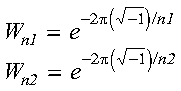
and where:
For scale = 1.0 and isign being positive, you obtain the discrete Fourier transform, a function of frequency. The inverse Fourier transform is obtained with scale = 1.0/((n1)(n2)) and isign being negative. See references [1], [4], and [20].
Two invocations of this subroutine are necessary:
Error 2015 is unrecoverable, naux2 = 0, and unable to allocate work area.
None
This example shows how to compute a two-dimensional transform where both input and output are stored in normal form (inc1x = inc1y = 1). Also, inc2x = inc2y so the same array can be used for both input and output. The arrays are declared as follows:
     COMPLEX*8  X(6,8),Y(6,8)
     REAL*8     AUX1(20000), AUX2(10000)
Arrays X and Y are made equivalent by the following statement, making them occupy the same storage: EQUIVALENCE (X,Y). First, initialize AUX1 using the calling sequence shown below with INIT <> 0. Then use the same calling sequence with INIT = 0 to do the calculation.
           INIT  X INC1X INC2X Y INC1Y INC2Y N1  N2 ISIGN SCALE  AUX1  NAUX1   AUX2  NAUX2
            |    |   |     |   |   |     |   |   |    |     |      |     |      |      |
CALL SCFT2(INIT, X , 1  ,  6 , Y , 1  ,  6 , 6 , 8 ,  1 , SCALE, AUX1, 20000 , AUX2, 10000)
INIT     =  1(for initialization)
INIT     =  0(for computation)
SCALE    =  1.0
X is an array with 6 rows and 8 columns with (1.0, 0.0) in all locations.
Y is an array with 6 rows and 8 columns having (48.0, 0.0) in location Y(1,1) and (0.0, 0.0) in all others.
This example shows how to compute a two-dimensional inverse Fourier transform. For this example, X is stored in normal untransposed form (inc1x = 1), and Y is stored in transposed form (inc2y = 1). The arrays are declared as follows:
     COMPLEX*16  X(6,8),Y(8,6)
     REAL*8      AUX1(20000), AUX2(10000)
First, initialize AUX1 using the calling sequence shown below with INIT <> 0. Then use the same calling sequence with INIT = 0 to do the calculation.
           INIT  X INC1X INC2X Y INC1Y INC2Y N1  N2 ISIGN SCALE  AUX1   NAUX1   AUX2   NAUX2
            |    |   |     |   |   |     |   |   |    |     |     |       |      |       |
CALL DCFT2(INIT, X , 1  ,  6 , Y , 8  ,  1 , 6 , 8 , -1 , SCALE, AUX1 , 20000 , AUX2 , 10000)
INIT     =  1(for initialization)
INIT     =  0(for computation)
SCALE    =  1.0/48.0
X        =(same as output Y in Example 1)
Y is an array with 8 rows and 6 columns with (1.0, 0.0) in all locations.
These subroutines compute the two-dimensional discrete Fourier transform of
real data in a two-dimensional array.
| X, scale | Y | Subroutine |
| Short-precision real | Short-precision complex | SRCFT2 |
| Long-precision real | Long-precision complex | DRCFT2 |
| Note: | Two invocations of this subroutine are necessary: one to prepare the working storage for the subroutine, and the other to perform the computations. |
| Fortran | CALL SRCFT2 (init, x, inc2x, y,
inc2y, n1, n2, isign, scale,
aux1, naux1, aux2, naux2, aux3,
naux3)
CALL DRCFT2 (init, x, inc2x, y, inc2y, n1, n2, isign, scale, aux1, naux1, aux2, naux2) |
| C and C++ | srcft2 (init, x, inc2x, y,
inc2y, n1, n2, isign, scale,
aux1, naux1, aux2, naux2, aux3,
naux3);
drcft2 (init, x, inc2x, y, inc2y, n1, n2, isign, scale, aux1, naux1, aux2, naux2); |
| PL/I | CALL SRCFT2 (init, x, inc2x, y,
inc2y, n1, n2, isign, scale,
aux1, naux1, aux2, naux2, aux3,
naux3);
CALL DRCFT2 (init, x, inc2x, y, inc2y, n1, n2, isign, scale, aux1, naux1, aux2, naux2); |
If init <> 0, trigonometric functions and other parameters, depending on arguments other than x, are computed and saved in aux1. The contents of x and y are not used or changed.
If init = 0, the discrete Fourier transform of the given array is computed. The only arguments that may change after initialization are x, y, and aux2. All scalar arguments must be the same as when the subroutine was called for initialization with init <> 0.
Specified as: a fullword integer. It can have any value.
If isign = positive value, Isign = + (transforming time to frequency).
If isign = negative value, Isign = - (transforming frequency to time).
Specified as: a fullword integer; isign > 0 or isign < 0.
If init <> 0, the working storage is computed.
If init = 0, the working storage is used in the computation of the Fourier transforms.
Specified as: an area of storage, containing naux1 long-precision real numbers.
If naux2 = 0 and error 2015 is unrecoverable, aux2 is ignored.
Otherwise, it is the working storage used by this subroutine, which is available for use by the calling program between calls to this subroutine.
Specified as: an area of storage, containing naux2 long-precision real numbers. On output, the contents are overwritten.
If naux2 = 0 and error 2015 is unrecoverable, SRCFT2 and DRCFT2 dynamically allocate the work area used by the subroutine. The work area is deallocated before control is returned to the calling program.
Otherwise, naux2 >= (minimum value required for successful processing). To determine a sufficient value, use the processor-independent formulas. For all other values specified less than the minimum value, you have the option of having the minimum value returned in this argument. For details, see "Using Auxiliary Storage in ESSL".
Specified as: an area of storage containing naux3 long-precision real numbers.
Specified as: a fullword integer.
If init <> 0, this argument is not used, and its contents remain unchanged.
If init = 0, this is array Y, containing the results of the complex discrete Fourier transform of X. The output consists of n2 columns of data. The data in each column is stored with stride 1. Due to complex conjugate symmetry, the output consists of only the first ((n1)/2)+1 rows of the array--that is, yk1,k2, where k1 = 0, 1, ..., (n1)/2 and k2 = 0, 1, ..., n2-1.
Returned as: an inc2y by (at least) n2 array, containing numbers of the data type indicated in Table 132. This array must be aligned on a doubleword boundary.
If init <> 0, it contains information ready to be passed in a subsequent invocation of this subroutine.
If init = 0, its contents are unchanged.
Returned as: the contents are not relevant.
The required values of naux1 and naux2 depend on n1 and n2.
The required values of naux1 and naux2 depend on n1 and n2.
The two-dimensional complex conjugate even discrete Fourier transform of real data in array X, with results going into array Y, is expressed as follows:
for:
where:
and where:
The output in array Y is complex. For scale = 1.0 and isign being positive, you obtain the discrete Fourier transform, a function of frequency. The inverse Fourier transform is obtained with scale = 1.0/((n1)(n2)) and isign being negative. See references [1], [4], [19], and [20].
Two invocations of this subroutine are necessary:
Error 2015 is unrecoverable, naux2 = 0, and unable to allocate work area.
None
This example shows how to compute a two-dimensional transform. The arrays are declared as follows:
     COMPLEX*8  Y(0:6,0:7)
     REAL*4     X(0:11,0:7)
     REAL*8     AUX1(1000), AUX2(1000), AUX3(1)
First, initialize AUX1 using the calling sequence shown below with INIT <> 0. Then use the same calling sequence with INIT = 0 to do the calculation.
            INIT  X  INC2X Y INC2Y N1  N2 ISIGN SCALE  AUX1   NAUX1  AUX2   NAUX2  AUX3  NAUX3
             |    |    |   |   |    |   |   |     |     |       |     |       |     |      |
CALL SRCFT2(INIT, X , 12 , Y , 7 , 12 , 8 , 1 , SCALE, AUX1 , 1000 , AUX2 , 1000 , AUX3 ,  0 )
INIT     =  1(for initialization)
INIT     =  0(for computation)
SCALE    =  1.0
X is an array with 12 rows and 8 columns having 1.0 in location X(0,0) and 0.0 in all others.
Y is an array with 7 rows and 8 columns with (1.0, 0.0) in all locations.
This example shows another transform computation with different data using the same initialized array AUX1 in Example 1.
            INIT X  INC2X Y INC2Y N1   N2 ISIGN SCALE  AUX1  NAUX1  AUX2  NAUX2  AUX3  NAUX3
             |   |    |   |   |   |    |    |     |     |      |     |      |     |      |
CALL SRCFT2( 0 , X , 12 , Y , 7 , 12 , 8 ,  1 , SCALE, AUX1, 1000 , AUX2, 1000 , AUX3 ,  0 )
SCALE    =  1.0
X is an array with 12 rows and 8 columns with 1.0 in all locations.
Y is an array with 7 rows and 8 columns having (96.0, 0.0) in location Y(0,0) and (0.0, 0.0) in all others.
This example shows the same array being used for input and output, where isign = -1 and scale = 1/((N1)(N2)). The arrays are declared as follows:
     COMPLEX*16  Y(0:8,0:7)
     REAL*8     X(0:19,0:7)
     REAL*8     AUX1(1000), AUX2(1000), AUX3(1)
Arrays X and Y are made equivalent by the following statement, making them occupy the same storage.
EQUIVALENCE (X,Y)
This requires inc2x >= 2(inc2y). First, initialize AUX1 using the calling sequence shown below with INIT <> 0. Then use the same calling sequence with INIT = 0 to do the calculation.
            INIT  X  INC2X Y INC2Y N1   N2 ISIGN SCALE  AUX1   NAUX1  AUX2   NAUX2  AUX3  NAUX3
             |    |    |   |   |   |    |    |      |     |      |     |       |     |      |
CALL DRCFT2(INIT, X , 20 , Y , 9 , 16 , 8 , -1 , SCALE, AUX1 , 1000 , AUX2 , 1000 , AUX3 ,  0 )
INIT     =  1(for initialization)
INIT     =  0(for computation)
SCALE    =  1.0/128.0
        *                                                *
        |  2.0   2.0  -2.0  -2.0   2.0   2.0  -2.0  -2.0 |
        |  2.0  -2.0  -2.0   2.0   2.0  -2.0  -2.0   2.0 |
        | -2.0  -2.0   2.0   2.0  -2.0  -2.0   2.0   2.0 |
        | -2.0   2.0   2.0  -2.0  -2.0   2.0   2.0  -2.0 |
        |  2.0   2.0  -2.0  -2.0   2.0   2.0  -2.0  -2.0 |
        |  2.0  -2.0  -2.0   2.0   2.0  -2.0  -2.0   2.0 |
        | -2.0  -2.0   2.0   2.0  -2.0  -2.0   2.0   2.0 |
        | -2.0   2.0   2.0  -2.0  -2.0   2.0   2.0  -2.0 |
        |  2.0   2.0  -2.0  -2.0   2.0   2.0  -2.0  -2.0 |
X    =  |  2.0  -2.0  -2.0   2.0   2.0  -2.0  -2.0   2.0 |
        | -2.0  -2.0   2.0   2.0  -2.0  -2.0   2.0   2.0 |
        | -2.0   2.0   2.0  -2.0  -2.0   2.0   2.0  -2.0 |
        |  2.0   2.0  -2.0  -2.0   2.0   2.0  -2.0  -2.0 |
        |  2.0  -2.0  -2.0   2.0   2.0  -2.0  -2.0   2.0 |
        | -2.0  -2.0   2.0   2.0  -2.0  -2.0   2.0   2.0 |
        | -2.0   2.0   2.0  -2.0  -2.0   2.0   2.0  -2.0 |
        |   .     .     .     .     .     .     .     .  |
        |   .     .     .     .     .     .     .     .  |
        |   .     .     .     .     .     .     .     .  |
        |   .     .     .     .     .     .     .     .  |
        *                                                *
Y is an array with 9 rows and 8 columns having (1.0, 1.0) in location Y(4,2) and (0.0, 0.0) in all others.
These subroutines compute the two-dimensional discrete Fourier transform of
complex conjugate even data in a two-dimensional array.
| X | Y, scale | Subroutine |
| Short-precision complex | Short-precision real | SCRFT2 |
| Long-precision complex | Long-precision real | DCRFT2 |
| Note: | Two invocations of this subroutine are necessary: one to prepare the working storage for the subroutine, and the other to perform the computations. |
| Fortran | CALL SCRFT2 (init, x, inc2x, y,
inc2y, n1, n2, isign, scale,
aux1, naux1, aux2, naux2, aux3,
naux3)
CALL DCRFT2 (init, x, inc2x, y, inc2y, n1, n2, isign, scale, aux1, naux1, aux2, naux2) |
| C and C++ | scrft2 (init, x, inc2x, y,
inc2y, n1, n2, isign, scale,
aux1, naux1, aux2, naux2, aux3,
naux3);
dcrft2 (init, x, inc2x, y, inc2y, n1, n2, isign, scale, aux1, naux1, aux2, naux2); |
| PL/I | CALL SCRFT2 (init, x, inc2x, y,
inc2y, n1, n2, isign, scale,
aux1, naux1, aux2, naux2, aux3,
naux3);
CALL DCRFT2 (init, x, inc2x, y, inc2y, n1, n2, isign, scale, aux1, naux1, aux2, naux2); |
If init <> 0, trigonometric functions and other parameters, depending on arguments other than x, are computed and saved in aux1. The contents of x and y are not used or changed.
If init = 0, the discrete Fourier transform of the given array is computed. The only arguments that may change after initialization are x, y, and aux2. All scalar arguments must be the same as when the subroutine was called for initialization with init <> 0.
Specified as: a fullword integer. It can have any value.
Specified as: an inc2x by (at least) n2 array, containing numbers of the data type indicated in Table 133. This array must be aligned on a doubleword boundary.
If isign = positive value, Isign = + (transforming time to frequency).
If isign = negative value, Isign = - (transforming frequency to time).
Specified as: a fullword integer; isign > 0 or isign < 0.
If init <> 0, the working storage is computed.
If init = 0, the working storage is used in the computation of the Fourier transforms.
Specified as: an area of storage, containing naux1 long-precision real numbers.
If naux2 = 0 and error 2015 is unrecoverable, aux2 is ignored.
Otherwise, it is the working storage used by this subroutine, which is available for use by the calling program between calls to this subroutine.
Specified as: an area of storage, containing naux2 long-precision real numbers. On output, the contents are overwritten.
If naux2 = 0 and error 2015 is unrecoverable, SCRFT2 and DCRFT2 dynamically allocate the work area used by the subroutine. The work area is deallocated before control is returned to the calling program.
Otherwise, naux2 >= (minimum value required for successful processing). To determine a sufficient value, use the processor-independent formulas. For all other values specified less than the minimum value, you have the option of having the minimum value returned in this argument. For details, see "Using Auxiliary Storage in ESSL".
Specified as: an area of storage, containing naux3 long-precision real numbers.
Specified as: a fullword integer.
If init <> 0, this argument is not used, and its contents remain unchanged.
If init = 0, this is the array Y, containing n1 rows and n2 columns of results of the real discrete Fourier transform of X. The data in each column of Y is stored with stride 1.
Returned as: an inc2y by (at least) n2 array, containing numbers of the data type indicated in Table 133. See "Notes" for more details.
If init <> 0, it contains information ready to be passed in a subsequent invocation of this subroutine.
If init = 0, its contents are unchanged.
Returned as: the contents are not relevant.
The required values of naux1 and naux2 depend on n1 and n2.
The required values of naux1 and naux2 depend on n1 and n2.
The two-dimensional discrete Fourier transform of complex conjugate even data in array X, with results going into array Y, is expressed as follows:
for:
where:
and where:
Because of the complex conjugate symmetry, the output in array Y is real. For scale = 1.0 and isign being positive, you obtain the discrete Fourier transform, a function of frequency. The inverse Fourier transform is obtained with scale = 1.0/((n1)(n2)) and isign being negative. See references [1], [4], and [20].
Two invocations of this subroutine are necessary:
Error 2015 is unrecoverable, naux2 = 0, and unable to allocate work area.
None
This example shows how to compute a two-dimensional transform. The arrays are declared as follows:
     REAL*4     Y(0:13,0:7)
     COMPLEX*8  X(0:6,0:7)
     REAL*8     AUX1(1000), AUX2(1000), AUX3(1)
First, initialize AUX1 using the calling sequence shown below with INIT <> 0. Then use the same calling sequence with INIT = 0 to do the calculation.
            INIT  X INC2X Y  INC2Y N1   N2 ISIGN SCALE   AUX1  NAUX1   AUX2  NAUX2   AUX3  NAUX3
             |    |   |   |    |   |    |    |     |      |      |      |      |      |      |
CALL SCRFT2(INIT, X , 7 , Y , 14 , 12 , 8 , -1 , SCALE , AUX1 , 1000 , AUX2 , 1000 , AUX3 ,  0 )
INIT     =  1(for initialization)
INIT     =  0(for computation)
SCALE    =  1.0/96.0
X is an array with 7 rows and 8 columns with (1.0, 0.0) in all locations.
        *                                        *
        | 1.0  0.0  0.0  0.0  0.0  0.0  0.0  0.0 |
        | 0.0  0.0  0.0  0.0  0.0  0.0  0.0  0.0 |
        | 0.0  0.0  0.0  0.0  0.0  0.0  0.0  0.0 |
        | 0.0  0.0  0.0  0.0  0.0  0.0  0.0  0.0 |
        | 0.0  0.0  0.0  0.0  0.0  0.0  0.0  0.0 |
        | 0.0  0.0  0.0  0.0  0.0  0.0  0.0  0.0 |
Y    =  | 0.0  0.0  0.0  0.0  0.0  0.0  0.0  0.0 |
        | 0.0  0.0  0.0  0.0  0.0  0.0  0.0  0.0 |
        | 0.0  0.0  0.0  0.0  0.0  0.0  0.0  0.0 |
        | 0.0  0.0  0.0  0.0  0.0  0.0  0.0  0.0 |
        | 0.0  0.0  0.0  0.0  0.0  0.0  0.0  0.0 |
        | 0.0  0.0  0.0  0.0  0.0  0.0  0.0  0.0 |
        |  .    .    .    .    .    .    .    .  |
        |  .    .    .    .    .    .    .    .  |
        *                                        *
This example shows another transform computation with different data using the same initialized array AUX1 in Example 1.
            INIT X INC2X Y  INC2Y N1   N2 ISIGN SCALE   AUX1   NAUX1  AUX2   NAUX2  AUX3  NAUX3
             |   |   |   |    |   |    |    |     |      |       |     |       |     |      |
CALL SCRFT2( 0 , X , 7 , Y , 14 , 12 , 8 , -1 , SCALE , AUX1 , 1000 , AUX2 , 1000 , AUX3 ,  0 )
SCALE = 1.0/96.0
X is an array with 7 rows and 8 columns having (96.0, 0.0) in location X(0,0) and (0.0, 0.0) in all others.
        *                                        *
        | 1.0  1.0  1.0  1.0  1.0  1.0  1.0  1.0 |
        | 1.0  1.0  1.0  1.0  1.0  1.0  1.0  1.0 |
        | 1.0  1.0  1.0  1.0  1.0  1.0  1.0  1.0 |
        | 1.0  1.0  1.0  1.0  1.0  1.0  1.0  1.0 |
        | 1.0  1.0  1.0  1.0  1.0  1.0  1.0  1.0 |
        | 1.0  1.0  1.0  1.0  1.0  1.0  1.0  1.0 |
Y    =  | 1.0  1.0  1.0  1.0  1.0  1.0  1.0  1.0 |
        | 1.0  1.0  1.0  1.0  1.0  1.0  1.0  1.0 |
        | 1.0  1.0  1.0  1.0  1.0  1.0  1.0  1.0 |
        | 1.0  1.0  1.0  1.0  1.0  1.0  1.0  1.0 |
        | 1.0  1.0  1.0  1.0  1.0  1.0  1.0  1.0 |
        | 1.0  1.0  1.0  1.0  1.0  1.0  1.0  1.0 |
        |  .    .    .    .    .    .    .    .  |
        |  .    .    .    .    .    .    .    .  |
        *                                        *
This example shows the same array being used for input and output. The arrays are declared as follows:
     REAL*8      Y(0:17,0:7)
     COMPLEX*16  X(0:8,0:7)
     REAL*8      AUX1(1000), AUX2(1000), AUX3(1)
Arrays X and Y are made equivalent by the following statement, making them occupy the same storage.
EQUIVALENCE (X,Y)
This requires inc2y = 2(inc2x). First, initialize AUX1 using the calling sequence shown below with INIT <> 0. Then use the same calling sequence with INIT = 0 to do the calculation.
            INIT  X INC2X Y  INC2Y N1  N2 ISIGN SCALE   AUX1   NAUX1  AUX2   NAUX2  AUX3  NAUX3
             |    |   |   |    |    |   |   |     |      |       |      |      |     |      |
CALL DCRFT2(INIT, X , 9 , Y , 18 , 16 , 8 , 1 , SCALE , AUX1 , 1000 , AUX2 , 1000 , AUX3 ,  0 )
INIT     =  1(for initialization)
INIT     =  0(for computation)
SCALE    =  1.0
X is an array with 9 rows and 8 columns having (1.0, 1.0) in location X(4,2) and (0.0, 0.0) in all others.
        *                                                *
        |  2.0   2.0  -2.0  -2.0   2.0   2.0  -2.0  -2.0 |
        |  2.0  -2.0  -2.0   2.0   2.0  -2.0  -2.0   2.0 |
        | -2.0  -2.0   2.0   2.0  -2.0  -2.0   2.0   2.0 |
        | -2.0   2.0   2.0  -2.0  -2.0   2.0   2.0  -2.0 |
        |  2.0   2.0  -2.0  -2.0   2.0   2.0  -2.0  -2.0 |
        |  2.0  -2.0  -2.0   2.0   2.0  -2.0  -2.0   2.0 |
        | -2.0  -2.0   2.0   2.0  -2.0  -2.0   2.0   2.0 |
        | -2.0   2.0   2.0  -2.0  -2.0   2.0   2.0  -2.0 |
Y    =  |  2.0   2.0  -2.0  -2.0   2.0   2.0  -2.0  -2.0 |
        |  2.0  -2.0  -2.0   2.0   2.0  -2.0  -2.0   2.0 |
        | -2.0  -2.0   2.0   2.0  -2.0  -2.0   2.0   2.0 |
        | -2.0   2.0   2.0  -2.0  -2.0   2.0   2.0  -2.0 |
        |  2.0   2.0  -2.0  -2.0   2.0   2.0  -2.0  -2.0 |
        |  2.0  -2.0  -2.0   2.0   2.0  -2.0  -2.0   2.0 |
        | -2.0  -2.0   2.0   2.0  -2.0  -2.0   2.0   2.0 |
        | -2.0   2.0   2.0  -2.0  -2.0   2.0   2.0  -2.0 |
        |   .     .     .     .     .     .     .     .  |
        |   .     .     .     .     .     .     .     .  |
        *                                                *
These subroutines compute the three-dimensional discrete Fourier transform of complex data.
| X, Y | scale | Subroutine |
| Short-precision complex | Short-precision real | SCFT3 |
| Long-precision complex | Long-precision real | DCFT3 |
| Note: | For each use, only one invocation of this subroutine is necessary. The initialization phase, preparing the working storage, is a relatively small part of the total computation, so it is performed on each invocation. |
| Fortran | CALL SCFT3 | DCFT3 (x, inc2x, inc3x, y, inc2y, inc3y, n1, n2, n3, isign, scale, aux, naux) |
| C and C++ | scft3 | dcft3 (x, inc2x, inc3x, y, inc2y, inc3y, n1, n2, n3, isign, scale, aux, naux); |
| PL/I | CALL SCFT3 | DCFT3 (x, inc2x, inc3x, y, inc2y, inc3y, n1, n2, n3, isign, scale, aux, naux); |
Specified as: an array, containing numbers of the data type indicated in Table 134. This array must be aligned on a doubleword boundary. If the array is dimensioned X(LDA1,LDA2,LDA3), then LDA1 = inc2x, (LDA1)(LDA2) = inc3x, and LDA3 >= n3. For information on how to set up this array, see "Setting Up Your Data". For more details, see "Notes".
If isign = positive value, Isign = + (transforming time to frequency).
If isign = negative value, Isign = - (transforming frequency to time).
Specified as: a fullword integer; isign > 0 or isign < 0.
If naux = 0 and error 2015 is unrecoverable, aux is ignored.
Otherwise, it is a storage work area used by this subroutine.
Specified as: an area of storage, containing naux long-precision real numbers. On output, the contents are overwritten.
If naux = 0 and error 2015 is unrecoverable, SCFT3 and DCFT3 dynamically allocate the work area used by the subroutine. The work area is deallocated before control is returned to the calling program.
Otherwise, naux >= (minimum value required for successful processing). To determine a sufficient value, use the processor-independent formulas. For all other values specified less than the minimum value, you have the option of having the minimum value returned in this argument. For details, see "Using Auxiliary Storage in ESSL".
Returned as: an array, containing numbers of the data type indicated in Table 134. This array must be aligned on a doubleword boundary. If the array is dimensioned Y(LDA1,LDA2,LDA3), then LDA1 = inc2y, (LDA1)(LDA2) = inc3y, and LDA3 >= n3. For information on how to set up this array, see "Setting Up Your Data". For more details, see "Notes".
If you specify different arrays X and Y, they must have no common elements; otherwise, results are unpredictable. See "Concepts".
Use the following formulas for calculating naux:
Use the following formulas for calculating naux:
The three-dimensional discrete Fourier transform of complex data in array X, with results going into array Y, is expressed as follows:
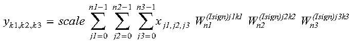
for:
where:
and where:
For scale = 1.0 and isign being positive, you obtain the discrete Fourier transform, a function of frequency. The inverse Fourier transform is obtained with scale = 1.0/((n1)(n2)(n3)) and isign being negative. See references [1], [4], [5], [19], and [20].
Error 2015 is unrecoverable, naux = 0, and unable to allocate work area.
None
This example shows how to compute a three-dimensional transform. In this example, INC2X >= INC2Y and INC3X >= INC3Y, so that the same array can be used for both input and output. The STRIDE subroutine is called to select good values for the INC2Y and INC3Y strides. (As explained below, STRIDE is not called for INC2X and INC3X.) Using the transform lengths (N1 = 32, N2 = 64, and N3 = 40) along with the output data type (short-precision complex: 'C'), STRIDE is called once for each stride needed. First, it is called for INC2Y:
CALL STRIDE (N2,N1,INC2Y,'C',0)
The output value returned for INC2Y is 32. Then STRIDE is called again for INC3Y:
CALL STRIDE (N3,N2*INC2Y,INC3Y,'C',0)
The output value returned for INC3Y is 2056. Because INC3Y is not a multiple of INC2Y, Y is not declared as a three-dimensional array. It is declared as a two-dimensional array, Y(INC3Y,N3).
To equivalence the X and Y arrays requires INC2X >= INC2Y and INC3X >= INC3Y. Therefore, INC2X is set equal to INC2Y( = 32). Also, to declare the X array as a three-dimensional array, INC3X must be a multiple of INC2X. Therefore, its value is set as INC3X = (65)(INC2X) = 2080.
The arrays are declared as follows:
     COMPLEX*8  X(32,65,40),Y(2056,40)
     REAL*8     AUX(30000)
Arrays X and Y are made equivalent by the following statement, making them occupy the same storage:
EQUIVALENCE (X,Y)
            X  INC2X INC3X  Y  INC2Y INC3Y  N1   N2   N3 ISIGN SCALE   AUX   NAUX
            |    |     |    |    |     |     |    |    |   |     |      |      |
CALL SCFT3( X , 32 , 2080 , Y , 32 , 2056 , 32 , 64 , 40 , 1 , SCALE , AUX , 30000)
SCALE    =  1.0
X has (1.0,2.0) in location X(1,1,1) and (0.0,0.0) in all other locations.
Y has (1.0,2.0) in locations Y(ij,k), where ij = 1, 2048 and j = 1, 40. It remains unchanged elsewhere.
These subroutines compute the three-dimensional discrete Fourier transform of real data in a three-dimensional array.
| X, scale | Y | Subroutine |
| Short-precision real | Short-precision complex | SRCFT3 |
| Long-precision real | Long-precision complex | DRCFT3 |
| Note: | For each use, only one invocation of this subroutine is necessary. The initialization phase, preparing the working storage, is a relatively small part of the total computation, so it is performed on each invocation. |
| Fortran | CALL SRCFT3 | DRCFT3 (x, inc2x, inc3x, y, inc2y, inc3y, n1, n2, n3, isign, scale, aux, naux) |
| C and C++ | srcft3 | drcft3 (x, inc2x, inc3x, y, inc2y, inc3y, n1, n2, n3, isign, scale, aux, naux); |
| PL/I | CALL SRCFT3 | DRCFT3 (x, inc2x, inc3x, y, inc2y, inc3y, n1, n2, n3, isign, scale, aux, naux); |
Specified as: an array, containing numbers of the data type indicated in Table 135. If the array is dimensioned X(LDA1,LDA2,LDA3), then LDA1 = inc2x, (LDA1)(LDA2) = inc3x, and LDA3 >= n3. For information on how to set up this array, see "Setting Up Your Data". For more details, see "Notes".
If isign = positive value, Isign = + (transforming time to frequency).
If isign = negative value, Isign = - (transforming frequency to time).
Specified as: a fullword integer; isign > 0 or isign < 0.
If naux = 0 and error 2015 is unrecoverable, aux is ignored.
Otherwise, it is a storage work area used by this subroutine.
Specified as: an area of storage, containing naux long-precision real numbers. On output, the contents are overwritten.
If naux = 0 and error 2015 is unrecoverable, SRCFT3 and DRCFT3 dynamically allocate the work area used by the subroutine. The work area is deallocated before control is returned to the calling program.
Otherwise, naux >= (minimum value required for successful processing). To determine a sufficient value, use the processor-independent formulas. For all other values specified less than the minimum value, you have the option of having the minimum value returned in this argument. For details, see "Using Auxiliary Storage in ESSL".
Returned as: an array, containing numbers of the data type indicated in Table 135. This array must be aligned on a doubleword boundary. If the array is dimensioned Y(LDA1,LDA2,LDA3), then LDA1 = inc2y, (LDA1)(LDA2) = inc3y, and LDA3 >= n3. For information on how to set up this array, see "Setting Up Your Data". For more details, see "Notes".
If you specify different arrays X and Y, they must have no common elements; otherwise, results are unpredictable. See "Concepts".
Use the following formulas for calculating naux:
If inc2x or inc3x is an odd number, or if array X is not aligned on a doubleword boundary, you should add the following amount to all the formulas given above:
Use the following formulas for calculating naux:
The three-dimensional complex conjugate even discrete Fourier transform of real data in array X, with results going into array Y, is expressed as follows:
for:
where:
and where:
The output in array Y is complex. For scale = 1.0 and isign being positive, you obtain the discrete Fourier transform, a function of frequency. The inverse Fourier transform is obtained with scale = 1.0/((n1)(n2)(n3)) and isign being negative. See references [1], [4], [5], [19], and [20].
Error 2015 is unrecoverable, naux = 0, and unable to allocate work area.
None
This example shows how to compute a three-dimensional transform. In this example, INC2X >= (2)(INC2Y) and INC3X >= (2)(INC3Y), so that the same array can be used for both input and output. The STRIDE subroutine is called to select good values for the INC2Y and INC3Y strides. Using the transform lengths (N1 = 32, N2 = 64, and N2 = 40) along with the output data type (short-precision complex: 'C'), STRIDE is called once for each stride needed. First, it is called for INC2Y:
CALL STRIDE (N2,N1/2+1,INC2Y,'C',0)
The output value returned for INC2Y is 17. (This value is equal to N1/2+1.) Then STRIDE is called again for INC3Y:
CALL STRIDE (N3,N2*INC2Y,INC3Y,'C',0)
The output value returned for INC3Y is 1088. Because INC3Y is a multiple of INC2Y--that is, INC3Y = (N2)(INC2Y)--Y is declared as a three-dimensional array, Y(17,64,40). (In general, for larger arrays, these types of values for INC2Y and INC3Y are not returned by STRIDE, and you are probably not able to declare Y as a three-dimensional array.)
To equivalence the X and Y arrays requires INC2X >= (2)(INC2Y) and INC3X >= (2)(INC3Y). Therefore, the values INC2X = (2)(INC2Y) = 34 and INC3X = (2)(INC3Y) = 2176 are set, and X is declared as a three-dimensional array, X(34,64,40).
The arrays are declared as follows:
     REAL*4     X(34,64,40)
     COMPLEX*8  Y(17,64,40)
     REAL*8     AUX(32000)
Arrays X and Y are made equivalent by the following statement, making them occupy the same storage:
EQUIVALENCE (X,Y)
             X  INC2X INC3X  Y  INC2Y INC3Y  N1   N2   N3 ISIGN SCALE   AUX    NAUX
             |    |     |    |    |     |     |    |    |   |     |      |      |
CALL SRCFT3( X , 34 , 2176 , Y , 17 , 1088 , 32 , 64 , 40 , 1 , SCALE , AUX , 32000)
SCALE    =  1.0
X has 1.0 in location X(1,1,1) and 0.0 in all other locations.
Y has (1.0,0.0) in all locations.
These subroutines compute the three-dimensional discrete Fourier transform
of complex conjugate even data in a three-dimensional array.
| X | Y, scale | Subroutine |
| Short-precision complex | Short-precision real | SCRFT2 |
| Long-precision complex | Long-precision real | DCRFT2 |
| Note: | For each use, only one invocation of this subroutine is necessary. The initialization phase, preparing the working storage, is a relatively small part of the total computation, so it is performed on each invocation. |
| Fortran | CALL SCRFT3 | DCRFT3 (x, inc2x, inc3x, y, inc2y, inc3y, n1, n2, n3, isign, scale, aux, naux) |
| C and C++ | scrft3 | dcrft3 (x, inc2x, inc3x, y, inc2y, inc3y, n1, n2, n3, isign, scale, aux, naux); |
| PL/I | CALL SCRFT3 | DCRFT3 (x, inc2x, inc3x, y, inc2y, inc3y, n1, n2, n3, isign, scale, aux, naux); |
Specified as: an array, containing numbers of the data type indicated in Table 136. This array must be aligned on a doubleword boundary. If the array is dimensioned X(LDA1,LDA2,LDA3), then LDA1 = inc2x, (LDA1)(LDA2) = inc3x, and LDA3 >= n3. For information on how to set up this array, see "Setting Up Your Data". For more details, see "Notes".
If isign = positive value, Isign = + (transforming time to frequency).
If isign = negative value, Isign = - (transforming frequency to time).
Specified as: a fullword integer; isign > 0 or isign < 0.
If naux = 0 and error 2015 is unrecoverable, aux is ignored.
Otherwise, it is a storage work area used by this subroutine. Specified as: an area of storage, containing naux long-precision real numbers. On output, the contents are overwritten.
If naux = 0 and error 2015 is unrecoverable, SCRFT3 and DCRFT3 dynamically allocate the work area used by the subroutine. The work area is deallocated before control is returned to the calling program.
Otherwise, naux >= (minimum value required for successful processing). To determine a sufficient value, use the processor-independent formulas. For all other values specified less than the minimum value, you have the option of having the minimum value returned in this argument. For details, see "Using Auxiliary Storage in ESSL".
Returned as: an array, containing numbers of the data type indicated in Table 136. If the array is dimensioned Y(LDA1,LDA2,LDA3), then LDA1 = inc2y, (LDA1)(LDA2) = inc3y, and LDA3 >= n3. For information on how to set up this array, see "Setting Up Your Data". For more details, see "Notes".
Use the following formulas for calculating naux:
If inc2y or inc3y is an odd number, or if array Y is not aligned on a doubleword boundary, you should add the following amount to all the formulas given above:
Use the following formulas for calculating naux:
The three-dimensional discrete Fourier transform of complex conjugate even data in array X, with results going into array Y, is expressed as follows:
for:
where:
and where:
Because of the complex conjugate symmetry, the output in array Y is real. For scale = 1.0 and isign being positive, you obtain the discrete Fourier transform, a function of frequency. The inverse Fourier transform is obtained with scale = 1.0/((n1)(n2)(n3)) and isign being negative. See references [1], [4], [5], [19], and [20].
Error 2015 is unrecoverable, naux = 0, and unable to allocate work area.
None
This example shows how to compute a three-dimensional transform. In this example, INC2Y = (2)(INC2X) and INC3Y = (2)(INC3X), so that the same array can be used for both input and output. The STRIDE subroutine is called to select good values for the INC2Y and INC3Y strides. (As explained below, STRIDE is not called for INC2X and INC3X.) Using the transform lengths (N1 = 32, N2 = 64, and N3 = 40) along with the output data type (short-precision real: 'S'), STRIDE is called once for each stride needed. First, it is called for INC2Y:
CALL STRIDE (N2,N1+2,INC2Y,'S',0)
The output value returned for INC2Y is 34. (This value is equal to N1+2.) Then STRIDE is called again for INC3Y:
CALL STRIDE (N3,N2*INC2Y,INC3Y,'S',0)
The output value returned for INC3Y is 2176. Because INC3Y is a multiple of INC2Y--that is, INC3Y = (N2)(INC2Y)--Y is declared as a three-dimensional array, Y(34,64,40). (In general, for larger arrays, these types of values for INC2Y and INC3Y are not returned by STRIDE, and you are probably not able to declare Y as a three-dimensional array.)
A good stride value for INC2X is INC2Y/2, and a good stride value for INC3X is INC3Y/2. Also, to equivalence the X and Y arrays requires INC2Y = (2)(INC2X) and INC3Y = (2)(INC3X). Therefore, the values INC2X = INC2Y/2 = 17 and INC3X = INC3Y/2 = 1088 are set, and X is declared as a three-dimensional array, X(17,64,40).
The arrays are declared as follows:
     COMPLEX*8  X(17,64,40)
     REAL*4     Y(34,64,40)
     REAL*8     AUX(32000)
Arrays X and Y are made equivalent by the following statement, making them occupy the same storage:
EQUIVALENCE (X,Y)
             X  INC2X INC3X  Y  INC2Y INC3Y  N1   N2   N3 ISIGN SCALE   AUX    NAUX
             |    |     |    |    |     |     |    |    |   |     |      |      |
CALL SCRFT3( X , 17 , 1088 , Y , 34 , 2176 , 32 , 64 , 40 , 1 , SCALE , AUX , 32000)
SCALE    =  1.0
X has (1.0,0.0) in location X(1,1,1) and (0.0,0.0) in all other locations.
Y has 1.0 in all locations.
This section contains the convolution and correlation subroutine descriptions.
These subroutines compute the convolutions and correlations of a sequence with one or more sequences using a direct method. The input and output sequences contain short-precision real numbers.
| Note: | These subroutines are considered obsolete. They are provided in ESSL only for compatibility with earlier releases. You should use SCOND, SCORD, SDCON, SDCOR, SCONF, and SCORF instead, because they provide better performance. For further details, see "Convolution and Correlation Considerations". |
| Fortran | CALL SCON | SCOR (init, h, inc1h, x, inc1x, inc2x, y, inc1y, inc2y, nh, nx, m, iy0, ny, aux1, naux1, aux2, naux2) |
| C and C++ | scon | scor (init, h, inc1h, x, inc1x, inc2x, y, inc1y, inc2y, nh, nx, m, iy0, ny, aux1, naux1, aux2, naux2); |
| PL/I | CALL SCON | SCOR (init, h, inc1h, x, inc1x, inc2x, y, inc1y, inc2y, nh, nx, m, iy0, ny, aux1, naux1, aux2, naux2); |
If init <> 0, no computation is performed, error checking is performed, and the subroutine exits back to the calling program.
If init = 0, the convolutions or correlations of the sequence in h with the sequences in x are computed.
Specified as: a fullword integer. It can have any value.
The convolutions and correlations of a sequence in array H with one or more sequences in array X are expressed as follows:
Convolutions for SCON:
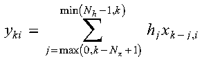
Correlations for SCOR:
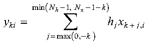
for:
where:
It is assumed that elements outside the range of definition are zero. See references [17] and [78].
Only one invocation of this subroutine is needed:
None
This example shows how to compute a convolution of a sequence in H, which is a ramp function, and three sequences in X, a triangular function and its cyclic translates. It computes the full range of nonzero values of the convolution plus two extra points, which are set to 0. The arrays are declared as follows:
     REAL*4   H(0:4999), X(0:49999), Y(0:49999)
     REAL*8   AUX1, AUX2
          INIT  H INC1H X INC1X INC2X Y INC1Y INC2Y NH NX  M IY0 NY  AUX1 NAUX1 AUX2 NAUX2
           |    |   |   |   |     |   |   |     |    |  |  |  |   |   |     |    |     |
CALL SCON(INIT, H , 1 , X , 1 ,  10 , Y , 1 ,  15 , 4, 10, 3, 0, 15, AUX1 , 0 , AUX2 , 0)
INIT     =  0(for computation)
H        =  (1.0, 2.0, 3.0, 4.0)
X contains the following three sequences:
1.0  2.0  3.0
2.0  1.0  2.0
3.0  2.0  1.0
4.0  3.0  2.0
5.0  4.0  3.0
6.0  5.0  4.0
5.0  6.0  5.0
4.0  5.0  6.0
3.0  4.0  5.0
2.0  3.0  4.0
Y contains the following three sequences:
 1.0   2.0   3.0
 4.0   5.0   8.0
10.0  10.0  14.0
20.0  18.0  22.0
30.0  20.0  18.0
40.0  30.0  20.0
48.0  40.0  30.0
52.0  48.0  40.0
50.0  52.0  48.0
40.0  50.0  52.0
29.0  38.0  47.0
18.0  25.0  32.0
 8.0  12.0  16.0
 0.0   0.0   0.0
 0.0   0.0   0.0
This example shows how the output from Example 1 differs when the values for NY and inc2y are 10 rather than 15. The output is the same except that it consists of only the first 10 values produced in Example 1.
Y contains the following three sequences:
 1.0   2.0   3.0
 4.0   5.0   8.0
10.0  10.0  14.0
20.0  18.0  22.0
30.0  20.0  18.0
40.0  30.0  20.0
48.0  40.0  30.0
52.0  48.0  40.0
50.0  52.0  48.0
40.0  50.0  52.0
This example shows how the output from Example 2 differs if the value for IY0 is 3 rather than 0. The output is the same except it starts at element 3 of the convolution sequences rather than element 0.
Y contains the following three sequences:
20.0  18.0  22.0
30.0  20.0  18.0
40.0  30.0  20.0
48.0  40.0  30.0
52.0  48.0  40.0
50.0  52.0  48.0
40.0  50.0  52.0
29.0  38.0  47.0
18.0  25.0  32.0
 8.0  12.0  16.0
This example shows how to compute a correlation of a sequence in H, which is a ramp function, and three sequences in X, a triangular function and its cyclic translates. It computes the full range of nonzero values of the correlation plus two extra points, which are set to 0. The arrays are declared as follows:
     REAL*4   H(0:4999), X(0:49999), Y(0:49999)
     REAL*8   AUX1, AUX2
          INIT  H INC1H X INC1X INC2X Y INC1Y INC2Y NH NX  M IY0  NY  AUX1  NAUX1 AUX2 NAUX2
           |    |   |   |   |     |   |   |     |   |  |   |   |   |   |      |    |     |
CALL SCOR(INIT, H , 1 , X , 1  , 10 , Y , 1  , 15 , 4, 10, 3, -3, 15, AUX1 ,  0 , AUX2 , 0)
INIT     =  0(for computation)
H        =  (1.0, 2.0, 3.0, 4.0)
X contains the following three sequences:
1.0  2.0  3.0
2.0  1.0  2.0
3.0  2.0  1.0
4.0  3.0  2.0
5.0  4.0  3.0
6.0  5.0  4.0
5.0  6.0  5.0
4.0  5.0  6.0
3.0  4.0  5.0
2.0  3.0  4.0
Y contains the following three sequences:
 4.0   8.0  12.0
11.0  10.0  17.0
20.0  15.0  16.0
30.0  22.0  18.0
40.0  30.0  22.0
50.0  40.0  30.0
52.0  50.0  40.0
48.0  52.0  50.0
40.0  48.0  52.0
30.0  40.0  48.0
16.0  22.0  28.0
 7.0  10.0  13.0
 2.0   3.0   4.0
 0.0   0.0   0.0
 0.0   0.0   0.0
This example shows how the output from Example 4 differs when the values for NY and INC2Y are 10 rather than 15. The output is the same except that it consists of only the first 10 values produced in Example 4.
Y contains the following three sequences:
 4.0   8.0  12.0
11.0  10.0  17.0
20.0  15.0  16.0
30.0  22.0  18.0
40.0  30.0  22.0
50.0  40.0  30.0
52.0  50.0  40.0
48.0  52.0  50.0
40.0  48.0  52.0
30.0  40.0  48.0
This example shows how the output from Example 5 differs if the value for IY0 is 0 rather than -3. The output is the same except it starts at element 0 of the correlation sequences rather than element -3.
Y contains the following three sequences:
30.0  22.0  18.0
40.0  30.0  22.0
50.0  40.0  30.0
52.0  50.0  40.0
48.0  52.0  50.0
40.0  48.0  52.0
30.0  40.0  48.0
16.0  22.0  28.0
 7.0  10.0  13.0
 2.0   3.0   4.0
These subroutines compute the convolution and correlation of a sequence with another sequence using a direct method. The input and output sequences contain short-precision real numbers.
Notes:
| Fortran | CALL SCOND | SCORD (h, inch, x, incx, y, incy, nh, nx, iy0, ny) |
| C and C++ | scond | scord (h, inch, x, incx, y, incy, nh, nx, iy0, ny); |
| PL/I | CALL SCOND | SCORD (h, inch, x, incx, y, incy, nh, nx, iy0, ny); |
The convolution and correlation of a sequence in array H with a sequence in array X are expressed as follows:
Convolution for SCOND:
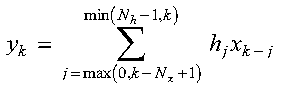
Correlation for SCORD:
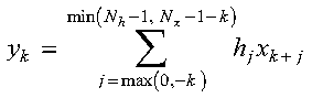
for k = iy0, iy0+1, ..., iy0+Ny-1
where:
It is assumed that elements outside the range of definition are zero. See reference [4].
SCORD can also perform the functions of SCON and SACOR; that is, it can compute convolutions and autocorrelations. To compute a convolution, you must specify a negative stride for H (see Example 9). To compute the autocorrelation, you must specify the two input sequences to be the same (see Example 10). In fact, you can also compute the autoconvolution by using both of these techniques together, letting the two input sequences be the same, and specifying a negative stride for the first input sequence.
None
This example shows how to compute a convolution of a sequence in H with a sequence in X, where both sequences are ramp functions.
            H  INCH  X  INCX  Y  INCY  NH  NX IY0  NY
            |   |    |   |    |   |    |   |   |   |
CALL SCOND( H , 1  , X , 1  , Y , 1  , 4 , 8 , 0 , 11 )

H        =  (1.0, 2.0, 3.0, 4.0)
X        =  (11.0, 12.0, 13.0, 14.0, 15.0, 16.0, 17.0, 18.0)
Y        =  (11.0, 34.0, 70.0, 120.0, 130.0, 140.0, 150.0, 160.0,
             151.0, 122.0, 72.0)
This example shows how the output from Example 1 differs when the value for IY0 is -2 rather than 0, and NY is 15 rather than 11. The output has two zeros at the beginning and end of the sequence, for points outside the range of nonzero output.
            H  INCH  X  INCX  Y  INCY  NH  NX  IY0  NY
            |   |    |   |    |   |    |   |    |   |
CALL SCOND( H , 1  , X , 1  , Y , 1  , 4 , 8 , -2 , 15 )

H        =  (1.0, 2.0, 3.0, 4.0)
X        =  (11.0, 12.0, 13.0, 14.0, 15.0, 16.0, 17.0, 18.0)
Y        =  (0.0, 0.0, 11.0, 34.0, 70.0, 120.0, 130.0, 140.0, 150.0,
             160.0, 151.0, 122.0, 72.0, 0.0, 0.0)
This example shows how the same output as Example 1 can be obtained when H and X are interchanged, because the convolution is symmetric in H and X. (The arguments are switched in the calling sequence.)
            H  INCH  X  INCX  Y  INCY  NH  NX IY0  NY
            |   |    |   |    |   |    |   |   |   |
CALL SCOND( X , 1  , H , 1  , Y , 1  , 4 , 8 , 0 , 11 )

H        =  (1.0, 2.0, 3.0, 4.0)
X        =  (11.0, 12.0, 13.0, 14.0, 15.0, 16.0, 17.0, 18.0)
Y        =  (11.0, 34.0, 70.0, 120.0, 130.0, 140.0, 150.0, 160.0,
             151.0, 122.0, 72.0)
This example shows how the output from Example 1 differs when a negative stride is specified for the sequence in H. By reversing the H sequence, the correlation is computed.
            H  INCH  X  INCX  Y  INCY  NH  NX IY0  NY
            |    |   |   |    |   |    |   |   |   |
CALL SCOND( H , -1 , X , 1  , Y , 1  , 4 , 8 , 0 , 11 )

H        =  (1.0, 2.0, 3.0, 4.0)
X        =  (11.0, 12.0, 13.0, 14.0, 15.0, 16.0, 17.0, 18.0)
Y        =  (44.0, 81.0, 110.0, 130.0, 140.0, 150.0, 160.0, 170.0,
             104.0, 53.0, 18.0)
This example shows how to compute the autoconvolution of a sequence by letting the two input sequences for H and X be the same. (X is specified for both arguments in the calling sequence.)
            H  INCH  X  INCX  Y  INCY NH  NX IY0  NY
            |   |   |   |    |   |    |   |   |   |
CALL SCOND( X , 1 , X , 1  , Y , 1  , 4 , 4 , 0 , 7 )

X        =  (11.0, 12.0, 13.0, 14.0)
Y = (121.0, 264.0, 430.0, 620.0, 505.0, 364.0, 196.0)
This example shows how to compute a correlation of a sequence in H with a sequence in X, where both sequences are ramp functions.
            H  INCH  X  INCX  Y  INCY NH  NX   IY0  NY
            |   |    |   |    |   |    |   |    |   |
CALL SCORD( H , 1  , X , 1  , Y , 1  , 4 , 8 , -3 , 11 )

H        =  (1.0, 2.0, 3.0, 4.0)
X        =  (11.0, 12.0, 13.0, 14.0, 15.0, 16.0, 17.0, 18.0)
Y        =  (44.0, 81.0, 110.0, 130.0, 140.0, 150.0, 160.0, 170.0,
             104.0, 53.0, 18.0)
This example shows how the output from Example 6 differs when the value for IY0 is -5 rather than -3 and NY is 15 rather than 11. The output has two zeros at the beginning and end of the sequence, for points outside the range of nonzero output.
            H  INCH  X  INCX  Y  INCY NH  NX   IY0  NY
            |   |    |   |    |   |    |   |    |   |
CALL SCORD( H , 1  , X , 1  , Y , 1  , 4 , 8 , -5 , 15 )

H        =  (1.0, 2.0, 3.0, 4.0)
X        =  (11.0, 12.0, 13.0, 14.0, 15.0, 16.0, 17.0, 18.0)
Y        =  (0.0, 0.0, 44.0, 81.0, 110.0, 130.0, 140.0, 150.0, 160.0,
             170.0, 104.0, 53.0, 18.0, 0.0, 0.0)
This example shows how the output from Example 6 differs when H and X are interchanged (in the calling sequence). The output sequence is the reverse of that in Example 6. To get the full range of output, IY0 is set to -NX+1.
            H  INCH  X  INCX  Y  INCY NH  NX   IY0  NY
            |   |    |   |    |   |    |   |    |   |
CALL SCORD( X , 1  , H , 1  , Y , 1  , 4 , 8 , -7 , 11 )

H        =  (1.0, 2.0, 3.0, 4.0)
X        =  (11.0, 12.0, 13.0, 14.0, 15.0, 16.0, 17.0, 18.0)
Y        =  (18.0, 53.0, 104.0, 170.0, 160.0, 150.0, 140.0, 130.0,
             110.0, 81.0, 44.0)
This example shows how the output from Example 6 differs when a negative stride is specified for the sequence in H. By reversing the H sequence, the convolution is computed.
            H  INCH  X  INCX  Y  INCY  NH  NX  IY0  NY
            |    |   |   |    |   |    |   |    |   |
CALL SCORD( H , -1 , X , 1  , Y , 1  , 4 , 8 , -3 , 11 )

H        =  (1.0, 2.0, 3.0, 4.0)
X        =  (11.0, 12.0, 13.0, 14.0, 15.0, 16.0, 17.0, 18.0)
Y        =  (11.0, 34.0, 70.0, 120.0, 130.0, 140.0, 150.0, 160.0,
             151.0, 122.0, 72.0)
This example shows how to compute the autocorrelation of a sequence by letting the two input sequences for H and X be the same. (X is specified for both arguments in the calling sequence.)
            H  INCH  X  INCX  Y  INCY  NH  NX  IY0  NY
            |   |    |   |    |   |    |   |    |   |
CALL SCORD( X , 1  , X , 1  , Y , 1  , 4 , 4 , -3 , 7 )

X        =  (11.0, 12.0, 13.0, 14.0)
Y = (154.0, 311.0, 470.0, 630.0, 470.0, 311.0, 154.0)
These subroutines compute the convolutions and correlations, respectively, of a sequence with one or more sequences using the mixed-radix Fourier method. The input and output sequences contain short-precision real numbers.
| Note: | Two invocations of these subroutines are necessary: one to prepare the working storage for the subroutine, and the other to perform the computations. |
| Fortran | CALL SCONF | SCORF (init, h, inc1h, x, inc1x, inc2x, y, inc1y, inc2y, nh, nx, m, iy0, ny, aux1, naux1, aux2, naux2) |
| C and C++ | sconf | scorf (init, h, inc1h, x, inc1x, inc2x, y, inc1y, inc2y, nh, nx, m, iy0, ny, aux1, naux1, aux2, naux2); |
| PL/I | CALL SCONF | SCORF (init, h, inc1h, x, inc1x, inc2x, y, inc1y, inc2y, nh, nx, m, iy0, ny, aux1, naux1, aux2, naux2); |
If init <> 0, trigonometric functions, the transform of the sequence in h, and other parameters, depending on arguments other than x, are computed and saved in aux1. The contents of x and y are not used or changed.
If init = 0, the convolutions or correlations of the sequence that was in h at initialization with the sequences in x are computed. h is not used or changed. The only arguments that may change after initialization are x, y, and aux2. All scalar arguments must be the same as when the subroutine was called for initialization with init <> 0.
Specified as: a fullword integer. It can have any value.
If init <> 0, the working storage is computed.
If init = 0, the working storage is used in the computation of the convolutions.
Specified as: an area of storage, containing naux1 long-precision real numbers.
If naux2 = 0 and error 2015 is unrecoverable, aux2 is ignored.
Otherwise, it is the working storage used by this subroutine, which is available for use by the calling program between calls to this subroutine.
Specified as: an area of storage, containing naux2 long-precision real numbers. On output, the contents are overwritten.
If naux2 = 0 and error 2015 is unrecoverable, SCONF and SCORF dynamically allocate the work area used by the subroutine. The work area is deallocated before control is returned to the calling program.
Otherwise, naux2 >= (minimum value required for successful processing). To determine a sufficient value, use the processor-independent formulas. For all other values specified less than the minimum value, you have the option of having the minimum value returned in this argument. For details, see "Using Auxiliary Storage in ESSL".
If init <> 0, this argument is not used, and its contents remain unchanged.
If init = 0, this is array Y, consisting of m output sequences of length Ny that are the result of the convolutions or correlations of the sequence in array H with the sequences in array X.
Returned as: an array of (at least) length 1+(Ny-1)inc1y+(m-1)inc2y, containing short-precision real numbers.
If init <> 0, it contains information ready to be passed in a subsequent invocation of this subroutine.
If init = 0, its contents are unchanged.
Returned as: the contents are not relevant.
Before calculating the necessary sizes of naux1 and naux2, you must determine the length n of the Fourier transform. The value of n is based on nf. You can use one of two techniques to determine nf:
After calculating the value for nf, using one of these two techniques, refer to the formula or table of allowable values of n in "Acceptable Lengths for the Transforms", selecting the value equal to or greater than nf.
The required values of naux1 and naux2 depend on the value determined for n in "Formulas for the Length of the Fourier Transform".
The convolutions and correlations of a sequence in array H with one or more sequences in array X are expressed as follows.
Convolutions for SCONF:
Correlations for SCORF:
for:
where:
These subroutines use a Fourier transform method with a mixed-radix capability. This provides maximum performance for your application. The length of the transform, n, that you must calculate to determine the correct sizes for naux1 and naux2 is the same length used by the Fourier transform subroutines called by this subroutine. It is assumed that elements outside the range of definition are zero. See references [17] and [78].
Two invocations of this subroutine are necessary:
Error 2015 is unrecoverable, naux2 = 0, and unable to allocate work area.
None
This example shows how to compute a convolution of a sequence in H, where H and X are ramp functions. It calculates all nonzero values of the convolution of the sequences in H and X. The arrays are declared as follows:
REAL*4 H(8), X(10,1), Y(17)
Because this convolution is symmetric in H and X, you can interchange the H and X sequences, leaving all other arguments the same, and you get the same output shown below. First, initialize AUX1 using the calling sequence shown below with INIT <> 0. Then use the same calling sequence with INIT = 0 to do the calculation.
           INIT  H INC1H X INC1X INC2X Y INC1Y INC2Y NH  NX  M IY0 NY  AUX1 NAUX1 AUX2 NAUX2
            |    |   |   |   |     |   |   |     |    |   |  |  |   |   |     |    |     |
CALL SCONF(INIT, H , 1 , X , 1  ,  1 , Y,  1  ,  1  , 8, 10, 1, 0, 17, AUX1, 128, AUX2, 23)
INIT     =  1(for initialization)
INIT     =  0(for computation)
H        =  (1.0, 2.0, 3.0, 4.0, 5.0, 6.0, 7.0, 8.0)
X        =  (11.0, 12.0, 13.0, 14.0, 15.0, 16.0, 17.0, 18.0, 19.0, 20.0)
Y        =  (11.0, 34.0, 70.0, 120.0, 185.0, 266.0, 364.0, 480.0,
             516.0, 552.0, 567.0, 560.0, 530.0, 476.0, 397.0, 292.0,
             160.0)
This example shows how the output from Example 1 differs when the value for NY is 21 rather than 17, and the value for IY0 is -2 rather than 0. This yields two zeros on each end of the convolution.
Y        =  (0.0, 0.0, 11.0, 34.0, 70.0, 120.0, 185.0, 266.0, 364.0,
             480.0, 516.0, 552.0, 567.0, 560.0, 530.0, 476.0, 397.0,
             292.0, 160.0, 0.0, 0.0)
This example shows how to compute the autoconvolution by letting the two input sequences be the same for Example 2. First, initialize AUX1 using the calling sequence shown below with INIT <> 0. Then use the same calling sequence with INIT = 0 to do the calculation.
           INIT  H INC1H X INC1X INC2X Y INC1Y INC2Y NH  NX  M  IY0  NY  AUX1 NAUX1 AUX2 NAUX2
            |    |   |   |   |     |   |   |     |    |   |  |   |    |   |     |    |     |
CALL SCONF(INIT, H , 1 , H , 1  ,  1 , Y,  1  ,  1  , 8, 10, 1, -2, 21, AUX1, 128, AUX2, 23)
INIT     =  1(for initialization)
INIT     =  0(for computation)
Y        =  (1.0, 4.0, 10.0, 20.0, 35.0, 56.0, 84.0, 120.0, 147.0,
             164.0, 170.0, 164.0, 145.0, 112.0, 64.0)
This example shows how to compute all nonzero values of the convolution of the sequence in H with the two sequences in X. First, initialize AUX1 using the calling sequence shown below with INIT <> 0. Then use the same calling sequence with INIT = 0 to do the calculation.
           INIT  H INC1H X INC1X INC2X Y INC1Y INC2Y NH  NX  M IY0 NY  AUX1 NAUX1 AUX2 NAUX2
            |    |   |   |   |     |   |   |     |    |   |  |  |   |   |     |    |     |
CALL SCONF(INIT, H , 1 , X,  1  , 10 , Y,  1  , 17  , 8, 10, 2, 0, 17, AUX1, 148, AUX2, 43)
INIT     =  1(for initialization)
INIT     =  0(for computation)
H        =  (1.0, 2.0, 3.0, 4.0, 5.0, 6.0, 7.0, 8.0)
X contains the following two sequences:
11.0  12.0
12.0  13.0
13.0  14.0
14.0  15.0
15.0  16.0
16.0  17.0
17.0  18.0
18.0  19.0
19.0  20.0
20.0  11.0
Y contains the following two sequences:
 11.0   12.0
 34.0   37.0
 70.0   76.0
120.0  130.0
185.0  200.0
266.0  287.0
364.0  392.0
480.0  516.0
516.0  552.0
552.0  578.0
567.0  582.0
560.0  563.0
530.0  520.0
476.0  452.0
397.0  358.0
292.0  237.0
160.0   88.0
This example shows how to compute a correlation of a sequence in H, where H and X are ramp functions. It calculates all nonzero values of the correlation of the sequences in H and X. The arrays are declared as follows:
REAL*4 H(8), X(10,1)
First, initialize AUX1 using the calling sequence shown below with INIT <> 0. Then use the same calling sequence with INIT = 0 to do the calculation.
           INIT  H INC1H X INC1X INC2X Y INC1Y INC2Y NH  NX  M  IY0 NY  AUX1 NAUX1 AUX2 NAUX2
            |    |   |   |   |     |   |   |     |    |   |  |   |   |   |     |    |     |
CALL SCORF(INIT, H , 1 , X,  1  ,  1 , Y,  1  ,  1  , 8, 10, 1, -7, 17, AUX1, 128, AUX2, 23)
INIT     =  1(for initialization)
INIT     =  0(for computation)
H        =(same as input H in Example 1)
X        =(same as input X in Example 1)
Y        =  (88.0, 173.0, 254.0, 330.0, 400.0, 463.0, 518.0, 564.0,
             600.0, 636.0, 504.0, 385.0, 280.0, 190.0, 116.0,
             59.0, 20.0)
This example shows how the output from Example 5 differs when the value for NY is 21 rather than 17, and the value for IY0 is -9 rather than 0. This yields two zeros on each end of the correlation.
Y        =  (0.0, 0.0, 88.0, 173.0, 254.0, 330.0, 400.0, 463.0, 518.0,
             564.0, 600.0, 636.0, 504.0, 385.0, 280.0, 190.0, 116.0,
             59.0, 20.0, 0.0, 0.0)
This example shows the effect of interchanging H and X. It uses the same input as Example 5, with H and X switched in the calling sequence, and with IY0 with a value of -9. Unlike convolution, as noted in Example 1, the correlation is not symmetric in H and X. First, initialize AUX1 using the calling sequence shown below with INIT <> 0. Then use the same calling sequence with INIT = 0 to do the calculation.
           INIT  H INC1H X INC1X INC2X Y INC1Y INC2Y NH  NX  M  IY0 NY  AUX1 NAUX1 AUX2 NAUX2
            |    |   |   |   |     |   |   |     |    |   |  |   |   |   |     |    |     |
CALL SCONF(INIT, X , 1 , H,  1  ,  1 , Y,  1  ,  1  , 8, 10, 1, -9, 17, AUX1, 128, AUX2, 23)
INIT     =  1(for initialization)
INIT     =  0(for computation)
Y        =  (20.0, 59.0, 116.0, 190.0, 280.0, 385.0, 504.0, 636.0,
             600.0, 564.0, 518.0, 463.0, 400.0, 330.0, 254.0, 173.0,
             88.0)
This example shows how to compute the autocorrelation by letting the two input sequences be the same. First, initialize AUX1 using the calling sequence shown below with INIT <> 0. Then use the same calling sequence with INIT = 0 to do the calculation. Because there is only one H input sequence, only one autocorrelation can be computed. Furthermore, this usage does not take advantage of the fact that the output is symmetric. Therefore, you should use SACORF to compute autocorrelations, because it does not have either of these problems.
           INIT  H INC1H X INC1X INC2X Y INC1Y INC2Y NH NX M  IY0 NY  AUX1 NAUX1 AUX2 NAUX2
            |    |   |   |   |     |   |   |     |   |  |  |   |   |   |     |    |     |
CALL SCONF(INIT, H , 1 , H,  1  ,  1 , Y,  1  ,  1 , 8, 8, 1, -7, 15, AUX1, 148, AUX2, 43)
INIT     =  1(for initialization)
INIT     =  0(for computation)
Y        =  (8.0, 23.0, 44.0, 70.0, 100.0, 133.0, 168.0, 204.0, 168.0,
             133.0, 100.0 , 70.0, 44.0, 23.0, 8.0)
This example shows how to compute all nonzero values of the correlation of the sequence in H with the two sequences in X. First, initialize AUX1 using the calling sequence shown below with INIT <> 0. Then use the same calling sequence with INIT = 0 to do the calculation.
           INIT  H INC1H X INC1X INC2X Y INC1Y INC2Y NH  NX  M  IY0 NY  AUX1 NAUX1 AUX2 NAUX2
            |    |   |   |   |     |   |   |     |    |   |  |   |   |   |     |    |     |
CALL SCONF(INIT, H , 1 , X,  1  , 10 , Y,  1  , 17  , 8, 10, 2, -7, 17, AUX1, 148, AUX2, 43)
INIT     =  1(for initialization)
INIT     =  0(for computation)
H        =(same as input H in Example 4)
X        =(same as input X in Example 4)
Y contains the following two sequences:
 88.0   96.0
173.0  188.0
254.0  275.0
330.0  356.0
400.0  430.0
463.0  496.0
518.0  553.0
564.0  600.0
600.0  636.0
636.0  592.0
504.0  462.0
385.0  346.0
280.0  245.0
190.0  160.0
116.0   92.0
 59.0   42.0
 20.0   11.0
These subroutines compute the convolution and correlation of a sequence
with another sequence, with decimated output, using a direct method.
| h, x, y | Subroutine |
| Short-precision real | SDCON |
| Long-precision real | DDCON |
| Short-precision real | SDCOR |
| Long-precision real | DDCOR |
| Note: | These subroutines are the short- and long-precision equivalents of SCOND and SCORD when the decimation interval id is equal to 1. Because there is no long-precision version of SCOND and SCORD, you can use DDCON and DDCOR, respectively, with decimation interval id = 1 to perform the same function. |
| Fortran | CALL SDCON | DDCON | SDCOR | DDCOR (h, inch, x, incx, y, incy, nh, nx, iy0, ny, id) |
| C and C++ | sdcon | ddcon | sdcor | ddcor (h, inch, x, incx, y, incy, nh, nx, iy0, ny, id); |
| PL/I | CALL SDCON | DDCON | SDCOR | DDCOR (h, inch, x, incx, y, incy, nh, nx, iy0, ny, id); |
Returned as: an array of (at least) length 1+(Ny-1)|incy|, containing numbers of the data type indicated in Table 137.
The convolution and correlation of a sequence in array H with a sequence in array X, with decimated output, are expressed as follows:
Convolution for SDCON and DDCON:
Correlation for SDCOR and DDCOR:
for k = iy0, iy0+id, iy0+(2)id, ..., iy0+(Ny-1)id
where:
It is assumed that elements outside the range of definition are zero. See reference [4].
SDCON and DDCON can also perform a correlation, autoconvolution, or autocorrelation. To compute a correlation, you must specify a negative stride for H. To compute the autoconvolution, you must specify the two input sequences to be the same. You can also compute the autocorrelation by using both of these techniques together, letting the two input sequences be the same, and specifying a negative stride for the first input sequence. For examples of this, see the examples for SCOND on page "Example 1". Because SCOND and SDCON are functionally the same, their results are the same as long as the decimation interval id = 1 for SDCON.
SDCOR and DDCOR can also perform a convolution, autocorrelation, or autoconvolution. To compute a convolution, you must specify a negative stride for H. To compute the autocorrelation, you must specify the two input sequences to be the same. You can also compute the autoconvolution by using both of these techniques together, letting the two input sequences be the same and specifying a negative stride for the first input sequence. For examples of these, see the examples for SCORD on page "Example 6". Because SCORD and SDCOR are functionally the same, their results are the same as long as the decimation interval id = 1 for SDCOR.
None
This example shows how to compute a convolution of a sequence in H with a sequence in X, where both sequences are ramp functions. It shows how a decimated output can be obtained, using the same input as "Example 1" for SCOND and using a decimation interval ID = 2.
| Note: | For further examples of use, see the examples for SCOND on page "Example 1". Because SCOND and SDCON are functionally the same, their results are the same as long as the decimation interval ID = 1 for SDCON. |
            H  INCH  X  INCX  Y  INCY  NH  NX IY0  NY  ID
            |   |    |   |    |   |    |   |   |   |   |
CALL SDCON( H , 1  , X , 1  , Y , 1  , 4 , 8 , 0 , 6 , 2 )

H        =  (1.0, 2.0, 3.0, 4.0)
X        =  (11.0, 12.0, 13.0, 14.0, 15.0, 16.0, 17.0, 18.0)
Y = (11.0, 70.0, 130.0, 150.0, 151.0, 72.0)
This example shows how to compute a correlation of a sequence in H with a sequence in X, where both sequences are ramp functions. It shows how a decimated output can be obtained, using the same input as "Example 6" for SCORD and using a decimation interval ID = 2.
| Note: | For further examples of use, see the examples for SCORD on page "Example 6". Because SCORD and SDCOR are functionally the same, their results are the same as long as the decimation interval ID = 1 for SDCOR. |
            H  INCH  X  INCX  Y  INCY  NH  NX  IY0  NY  ID
            |   |    |   |    |   |    |   |    |   |   |
CALL SDCOR( H , 1  , X , 1  , Y , 1  , 4 , 8 , -3 , 6 , 2 )

H        =  (1.0, 2.0, 3.0, 4.0)
X        =  (11.0, 12.0, 13.0, 14.0, 15.0, 16.0, 17.0, 18.0)
Y = (44.0, 110.0, 140.0, 160.0, 104.0, 18.0)
This example shows how to compute the same function as computed in "Example 1" for SCOND. The input sequences and arguments are the same as that example, except a decimation interval ID = 1 is specified here for SDCON.
            H  INCH  X  INCX  Y  INCY  NH  NX IY0  NY   ID
            |   |    |   |    |   |    |   |   |    |   |
CALL SDCON( H , 1  , X , 1  , Y , 1  , 4 , 8 , 0 , 11 , 1 )

H        =  (1.0, 2.0, 3.0, 4.0)
X        =  (11.0, 12.0, 13.0, 14.0, 15.0, 16.0, 17.0, 18.0)
Y        =  (11.0, 34.0, 70.0, 120.0, 130.0, 140.0, 150.0, 160.0,
             151.0, 122.0, 72.0)
This subroutine computes the autocorrelations of one or more sequences using a direct method. The input and output sequences contain short-precision real numbers.
| Note: | This subroutine is considered obsolete. It is provided in ESSL only for compatibility with earlier releases. You should use SCORD, SDCOR, SCORF and SACORF instead, because they provide better performance. For further details, see reference [4]. |
| Fortran | CALL SACOR (init, x, inc1x, inc2x, y, inc1y, inc2y, nx, m, ny, aux1, naux1, aux2, naux2) |
| C and C++ | sacor (init, x, inc1x, inc2x, y, inc1y, inc2y, nx, m, ny, aux1, naux1, aux2, naux2); |
| PL/I | CALL SACOR (init, x, inc1x, inc2x, y, inc1y, inc2y, nx, m, ny, aux1, naux1, aux2, naux2); |
If init <> 0, no computation is performed, error checking is performed, and the subroutine exits back to the calling program.
If init = 0, the autocorrelations of the sequence in x are computed.
Specified as: a fullword integer. It can have any value.
The autocorrelations of the sequences in array X are expressed as follows:

for:
where:
Only one invocation of this subroutine is needed:
None
This example shows how to compute an autocorrelation for three short sequences in array X, where the input sequence length NX is equal to the output sequence length NY. This gives all nonzero autocorrelation values.
The arrays are declared as follows:
     REAL*4   X(0:49999), Y(0:49999)
     REAL*8   AUX1, AUX2
           INIT  X INC1X INC2X Y INC1Y INC2Y NX  M   NY  AUX1 NAUX1 AUX2   NAUX2
            |    |   |     |   |   |     |   |   |   |    |     |    |       |
CALL SACOR(INIT, X , 1  ,  7 , Y , 1  ,  7 , 7 , 3 , 7 , AUX1 , 0 , AUX2 ,   0)
INIT = 0(for computation)
X contains the following three sequences:
1.0  2.0  3.0
2.0  1.0  2.0
3.0  2.0  1.0
4.0  3.0  2.0
4.0  4.0  3.0
3.0  4.0  4.0
2.0  3.0  4.0
Y contains the following three sequences:
59.0  59.0  59.0
54.0  50.0  44.0
43.0  39.0  30.0
29.0  27.0  24.0
16.0  18.0  21.0
 7.0  11.0  20.0
 2.0   6.0  12.0
This example shows how the output from Example 1 differs when the values for NY and INC2Y are 9 rather than 7. This shows that when NY is greater than NX, the output array is longer, and that part is filled with zeros.
Y contains the following three sequences:
59.0  59.0  59.0
54.0  50.0  44.0
43.0  39.0  30.0
29.0  27.0  24.0
16.0  18.0  21.0
 7.0  11.0  20.0
 2.0   6.0  12.0
 0.0   0.0   0.0
 0.0   0.0   0.0
This example shows how the output from Example 1 differs when the value for NY is 5 rather than 7. Also, the values for INC1X and INC1Y are 3, and the values for INC2X and INC2Y are 1 rather than 7. This shows that when NY is less than NX, the output array is shortened.
Y contains the following three sequences:
59.0  59.0  59.0
54.0  50.0  44.0
43.0  39.0  30.0
29.0  27.0  24.0
16.0  18.0  21.0
This subroutine computes the autocorrelations of one or more sequences using the mixed-radix Fourier method. The input and output sequences contain short-precision real numbers.
| Note: | Two invocations of this subroutine are necessary: one to prepare the working storage for the subroutine, and the other to perform the computations. |
| Fortran | CALL SACORF (init, x, inc1x, inc2x, y, inc1y, inc2y, nx, m, ny, aux1, naux1, aux2, naux2) |
| C and C++ | sacorf (init, x, inc1x, inc2x, y, inc1y, inc2y, nx, m, ny, aux1, naux1, aux2, naux2); |
| PL/I | CALL SACORF (init, x, inc1x, inc2x, y, inc1y, inc2y, nx, m, ny, aux1, naux1, aux2, naux2); |
If init <> 0, trigonometric functions and other parameters, depending on arguments other than x, are computed and saved in aux1. The contents of x and y are not used or changed.
If init = 0, the autocorrelations of the sequence in x are computed. The only arguments that may change after initialization are x, y, and aux2. All scalar arguments must be the same as when the subroutine was called for initialization with init <> 0.
Specified as: a fullword integer. It can have any value.
If init <> 0, the working storage is computed.
If init = 0, the working storage is used in the computation of the autocorrelations.
Specified as: an area of storage, containing naux1 long-precision real numbers.
If naux2 = 0 and error 2015 is unrecoverable, aux2 is ignored.
Otherwise, it is the working storage used by this subroutine, which is available for use by the calling program between calls to this subroutine.
Specified as: an area of storage, containing naux2 long-precision real numbers. On output, the contents are overwritten.
If naux2 = 0 and error 2015 is unrecoverable, SACORF dynamically allocates the work area used by this subroutine. The work area is deallocated before control is returned to the calling program.
Otherwise, naux2 >= (minimum value required for successful processing). To determine a sufficient value, use the processor-independent formulas. For all other values specified less than the minimum value, you have the option of having the minimum value returned in this argument. For details, see "Using Auxiliary Storage in ESSL".
If init <> 0, this argument is not used, and its contents remain unchanged.
If init = 0, this is array Y, consisting of m output sequences of length Ny that are the autocorrelation functions of the sequences in array X.
Returned as: an array of (at least) length 1+(Ny-1)inc1y+(m-1)inc2y, containing short-precision real numbers.
If init <> 0, it contains information ready to be passed in a subsequent invocation of this subroutine.
If init = 0, its contents are unchanged.
Returned as: the contents are not relevant.
Before calculating the necessary sizes of naux1 and naux2, you must determine the length n of the Fourier transform. To do this, you use the values of the arguments nx and ny, inserted into the following formula, to get a value for the variable nf. After calculating nf, reference the formula or table of allowable values of n in "Acceptable Lengths for the Transforms", selecting the value equal to or greater than nf. Following is the formula for determining nf:
The required values of naux1 and naux2 depend on the value determined for n in "Formula for Calculating the Length of the Fourier Transform" and the argument m.
The autocorrelations of the sequences in array X are expressed as follows:
for:
where:
This subroutine uses a Fourier transform method with a mixed-radix capability. This provides maximum performance for your application. The length of the transform, n, that you must calculate to determine the correct sizes for naux1 and naux2 is the same length used by the Fourier transform subroutines called by this subroutine. See references [17] and [78].
Two invocations of this subroutine are necessary:
Error 2015 is unrecoverable, naux2 = 0, and unable to allocate work area.
None
This example shows how to compute an autocorrelation for three short sequences in array X, where the input sequence length NX is equal to the output sequence length NY. This gives all nonzero autocorrelation values. The arrays are declared as follows:
     REAL*4   X(0:49999), Y(0:49999)
     REAL*8   AUX1(30788), AUX2(17105)
First, initialize AUX1 using the calling sequence shown below with INIT <> 0. Then use the same calling sequence with INIT = 0 to do the calculation.
            INIT  X INC1X INC2X Y INC1Y INC2Y NX  M   NY  AUX1  NAUX1 AUX2  NAUX2
             |    |   |     |   |   |     |   |   |   |    |      |    |      |
CALL SACORF(INIT, X , 1  ,  7 , Y , 1  ,  7 , 7 , 3 , 7 , AUX1, 2959, AUX2, 4354)
INIT     =  1(for initialization)
INIT     =  0(for computation)
X contains the following three sequences:
1.0  2.0  3.0
2.0  1.0  2.0
3.0  2.0  1.0
4.0  3.0  2.0
4.0  4.0  3.0
3.0  4.0  4.0
2.0  3.0  4.0
Y contains the following three sequences:
59.0  59.0  59.0
54.0  50.0  44.0
43.0  39.0  30.0
29.0  27.0  24.0
16.0  18.0  21.0
 7.0  11.0  20.0
 2.0   6.0  12.0
This example shows how the output from Example 1 differs when the value for NY and INC2Y are 9 rather than 7. This shows that when NY is greater than NX, the output array is longer and that part is filled with zeros.
Y contains the following three sequences:
59.0  59.0  59.0
54.0  50.0  44.0
43.0  39.0  30.0
29.0  27.0  24.0
16.0  18.0  21.0
 7.0  11.0  20.0
 2.0   6.0  12.0
 0.0   0.0   0.0
 0.0   0.0   0.0
This example shows how the output from Example 1 differs when the value for NY is 5 rather than 7. Also, the values for INC1X and INC1Y are 3 rather than 1, and the values for INC2X and INC2Y are 1 rather than 7. This shows that when NY is less than NX, the output array is shortened.
Y contains the following three sequences:
59.0  59.0  59.0
54.0  50.0  44.0
43.0  39.0  30.0
29.0  27.0  24.0
16.0  18.0  21.0
This section contains the related-computation subroutine descriptions.
These subroutines evaluate a polynomial of degree k, using coefficient vector u, input vector x, and output vector y:

where uk, xi, and
yi are elements of u, x,
and y, respectively.
| u, x, y | Subroutine |
|---|---|
| Short-precision real | SPOLY |
| Long-precision real | DPOLY |
| Fortran | CALL SPOLY | DPOLY (u, incu, k, x, incx, y, incy, n) |
| C and C++ | spoly | dpoly (u, incu, k, x, incx, y, incy, n); |
| PL/I | CALL SPOLY | DPOLY (u, incu, k, x, incx, y, incy, n); |
Vectors u, x, and y must have no common elements; otherwise, results are unpredictable. See "Concepts".
The evaluation of the polynomial:
is expressed as follows:
See reference [75] for Horner's Rule. If n is 0, no computation is performed. For SPOLY, intermediate results are accumulated in long precision.
SPOLY provides the same function as the IBM 3838 function POLY, with restrictions removed. DPOLY provides a long-precision computation that is not included in the IBM 3838 functions. See the IBM 3838 Array Processor Functional Characteristics manual.
None
This example shows a polynomial evaluation with the degree, K, equal to 0.
            U   INCU   K   X   INCX   Y  INCY  N
            |    |     |   |    |     |   |    |
CALL SPOLY( U , INCU , 0 , X , INCX , Y , 1  , 3 )
U        =  (4.0)
INCU     =(not relevant)
X        =(not relevant)
INCX     =(not relevant)
Y = (4.0, 4.0, 4.0)
This example shows a polynomial evaluation, using a negative stride INCU for vector u. For u, processing begins at element U(4) which is 1.0.
            U  INCU  K   X  INCX  Y  INCY  N
            |    |   |   |   |    |   |    |
CALL SPOLY( U , -1 , 3 , X , 1  , Y , 1  , 3 )

U        =  (4.0, 3.0, 2.0, 1.0)
X        =  (2.0, 1.0, -3.0)
Y = (49.0, 10.0, -86.0)
This example shows a polynomial evaluation, using a stride INCX of 0 for input vector x.
            U  INCU  K   X  INCX  Y  INCY  N
            |   |    |   |   |    |   |    |
CALL SPOLY( U , 1  , 3 , X , 0  , Y , 1  , 3 )

U        =  (4.0, 3.0, 2.0, 1.0)
X        =  (2.0, . , . )
Y = (26.0, 26.0, 26.0)
This example shows a polynomial evaluation, using a stride INCX greater than 1 for input vector x, and a negative stride INCY for output vector y. For y, results are stored beginning at element Y(5).
            U  INCU  K   X  INCX  Y  INCY  N
            |   |    |   |   |    |    |   |
CALL SPOLY( U , 1  , 3 , X , 2  , Y , -2 , 3 )

U        =  (4.0, 3.0, 2.0, 1.0)
X        =  (2.0, . , -3.0, . , 1.0)
Y = (10.0, . , -14.0, . , 26.0)
These subroutines find the position of the i-th zero crossing in
vector x. This is the i-th transition between positive and
negative or negative and positive, where 0 is considered a positive value. It
returns the position of the element in vector x where the
i-th zero crossing is detected. The direction of the scan is either
from the first element to the last or from the last element to the first,
depending on the value you specify for the scan direction argument.
| x | Subroutine |
|---|---|
| Short-precision real | SIZC |
| Long-precision real | DIZC |
| Fortran | CALL SIZC | DIZC (x, idrx, n, i, ky) |
| C and C++ | sizc | dizc (x, idrx, n, i, ky); |
| PL/I | CALL SIZC | DIZC (x, idrx, n, i, ky); |
If the i-th zero crossing is found:
If the i-th zero crossing is not found:
Returned as: an array of (at least) length 2, containing fullword integers.
The aux and naux arguments, required in some earlier releases of ESSL, are no longer required by these subroutines. If your program still includes them, you do not have to change your program; it continues to run normally. It ignores these arguments. However, if you did any program checking for error code 2015, you may want to remove it, because this error no longer occurs. (You must not code these arguments in your C program.)
The i-th zero crossing in vector x is found by scanning vector x for i occurrences of TRUE for the following logical expressions. A zero crossing is defined here as a crossing either from a positive value to a negative value or from a negative value to a positive value, where 0 is considered a positive value. If the i-th zero crossing is found, the value of j at that point is returned in ky1 as the position of the i-th zero crossing, and i is returned in ky2.
If idrx >= 0:
If idrx < 0:
If the position of the i-th zero crossing is not found, 0 is returned in y1 and the number of zero crossings encountered in the scan is returned in y2.
SIZC provides the same functions as the IBM 3838 functions NZCP and NZCN, with restrictions removed. It combines these functions into one ESSL subroutine. DIZC provides a long-precision computation that is not included in the IBM 3838 functions. See the IBM 3838 Array Processor Functional Characteristics manual.
None
This example shows a scan of a vector x from the first element to the last. It is looking for the fifth zero crossing, which is encountered at position 9.
           X  IDRX  N    I   KY
           |   |    |    |   |
CALL SIZC( X , 1  , 12 , 5 , KY )

X        =  (2.0, -1.0, -3.0, 3.0, 0.0, 8.0, -2.0, 0.0, -5.0, -3.0,
             2.0, -9.0)
KY = (9, 5)
This example shows a scan of a vector x from the last element to the first. It is looking for the seventh zero crossing, which is encountered at position 3. Because IDRX is negative, X is scanned from the last element, X(12), to the first element, X(1).
           X  IDRX  N    I   KY
           |    |   |    |   |
CALL SIZC( X , -1 , 12 , 7 , KY )

X        =  (2.0, -1.0, 3.0, -3.0, 0.0, -8.0, -2.0, 0.0, -5.0, -3.0,
             2.0, -9.0)
KY = (3, 7)
This example shows a scan of a vector x when the i-th zero crossing is not found. It encounters seven zero crossings and returns this value in KY(2).
           X  IDRX  N    I    KY
           |   |    |    |    |
CALL SIZC( X , 1  , 12 , 10 , KY )

X        =  (2.0, -1.0, -3.0, 3.0, 0.0, 8.0, -2.0, 0.0, -5.0, -3.0,
             2.0, -9.0)
KY = (0, 7)
These subroutines implement the first-order time-varying recursive
equation, using initial value s, target vectors u and
x, and output vector y.
| s, u, x, y | Subroutine |
|---|---|
| Short-precision real | STREC |
| Long-precision real | DTREC |
| Fortran | CALL STREC | DTREC (s, u, incu, x, incx, y, incy, n , iopt) |
| C and C++ | strec | dtrec (s, u, incu, x, incx, y, incy, n, iopt); |
| PL/I | CALL STREC | DTREC (s, u, incu, x, incx, y, incy, n , iopt); |
Vectors u, x, and y must have no common elements; otherwise, results are unpredictable. See "Concepts".
The first-order time-varying recursive equation is expressed as follows:
STREC provides the same function as the IBM 3838 function REC, with restrictions removed. DTREC provides a long-precision computation that is not included in the IBM 3838 functions. See the IBM 3838 Array Processor Functional Characteristics manual.
None
This example shows all strides INCU, INCX, and INCY equal to 1 for vectors u, x, and y, respectively.
             S    U  INCU  X  INCX  Y  INCY  N  IOPT
             |    |   |    |   |    |   |    |   |
CALL STREC( 1.0 , U , 1  , X , 1  , Y , 1  , 8 , 0 )

U        =  (1.0, 2.0, 3.0, 3.0, 2.0, 1.0, 1.0, 2.0)
X        =  (3.0, 2.0, 1.0, 1.0, 2.0, 3.0, 3.0, 2.0)
Y = (4.0, 10.0, 31.0, 94.0, 190.0, 193.0, 196.0, 394.0)
This example shows a stride, INCU, that is greater than 1 for vector u. The strides INCX and INCY for vectors x and y, respectively, are 1.
             S    U  INCU  X  INCX  Y  INCY  N  IOPT
             |    |   |    |   |    |   |    |   |
CALL STREC( 1.0 , U , 2  , X , 1  , Y , 1  , 4 , 0 )

U        =  (1.0, . , 3.0, . , 2.0, . , 1.0, . )
X        =  (3.0, 2.0, 1.0, 1.0, 2.0, 3.0, 3.0, 2.0)
Y = (4.0, 14.0, 29.0, 30.0)
This example shows a stride, INCU, of 1 for vector u, a stride, INCX, that is greater than 1 for vector x, and a negative stride, INCY, for vector y. For y, results are stored beginning at element Y(4).
             S    U  INCU  X  INCX  Y  INCY  N  IOPT
             |    |   |    |   |    |    |   |   |
CALL STREC( 1.0 , U , 1  , X , 2  , Y , -1 , 4 , 1 )

U        =  (1.0, 2.0, 3.0, 3.0, 2.0, 1.0, 1.0, 2.0)
X        =  (3.0, . , 1.0, . , 2.0, . , 3.0)
Y = (90.0, 29.0, 9.0, 4.0)
These subroutines perform a quadratic interpolation at specified points in
the vector x, using initial linear displacement in the samples
s, sample interval g, output scaling parameter OMEGA, and
sample reflection times in vector t. The result is returned in
vector y.
| x, s, g, OMEGA, t, y | Subroutine |
|---|---|
| Short-precision real | SQINT |
| Long-precision real | DQINT |
| Fortran | CALL SQINT | DQINT (s, g, omega, x, incx, n, t, inct, y, incy, m) |
| C and C++ | sqint | dqint (s, g, omega, x, incx, n, t, inct, y, incy, m); |
| PL/I | CALL SQINT | DQINT (s, g, omega, x, incx, n, t, inct, y, incy, m); |
The quadratic interpolation, which is expressed as follows:

uses the following values:
and where trace, k, f, and w are four working vectors, and so is a working scalar defined as:
| Note: | Allowing ki+1 to have a value of 2 results in performance degradation. If possible, avoid specifying a point at which this occurs. |
If n or m is 0, no computation is performed.
SQINT provides the same function as the IBM 3838 function INT, with restrictions removed. DQINT provides a long-precision computation that is not included in the IBM 3838 functions. See the IBM 3838 Array Processor Functional Characteristics manual.
The condition (ki+1 > n) or (ki+1 <= 2) has occurred, where n is the number of elements in vector x. See "Function" for how to calculate ki.
This example shows a quadratic interpolation, using vectors with strides of 1.
             S     G   OMEGA  X  INCX  N   T  INCT  Y  INCY  M
             |     |     |    |   |    |   |   |    |   |    |
CALL SQINT( 2.0 , 1.0 , 1.0 , X , 1  , 8 , T , 1  , Y , 1  , 4 )

X        =  (1.0, 2.0, 3.0, 4.0, 5.0, 6.0, 7.0, 8.0)
T        =  (1.5, 2.5, 3.5, 4.5)
Y = (9.0, 11.0, 13.0, 15.0)
This example shows a quadratic interpolation, using vectors with a positive stride of 1 and negative strides of -1.
             S     G   OMEGA  X  INCX  N   T  INCT  Y  INCY  M
             |     |     |    |    |   |   |    |   |   |    |
CALL SQINT( 2.0 , 1.0 , 1.0 , X , -1 , 8 , T , -1 , Y , 1  , 4 )

X        =  (1.0, 2.0, 3.0, 4.0, 5.0, 6.0, 7.0, 8.0)
T        =  (1.5, 2.5, 3.5, 4.5)
Y = (3.0, 5.0, 7.0, 9.0)
This example shows a quadratic interpolation, using vectors with a positive stride greater than 1 and negative strides less than -1.
             S     G   OMEGA  X  INCX  N   T  INCT  Y  INCY  M
             |     |     |    |    |   |   |    |   |   |    |
CALL SQINT( 2.0 , 1.0 , 1.0 , X , -2 , 8 , T , -1 , Y , 2  , 4 )

X        =  (1.0, . , 3.0, . , 5.0, . , 7.0, . , 9.0, . , 11.0, . ,
             13.0, . , 15.0)
T        =  (1.36, 2.36, 3.36, 4.36)
Y = (4.56, . , 8.56, . , 12.56, . , 16.56)
This example shows a quadratic interpolation, using vectors with positive strides and larger values for S and G than shown in the previous examples.
             S      G   OMEGA  X  INCX  N   T  INCT  Y  INCY  M
             |      |     |    |   |    |   |   |    |   |    |
CALL SQINT( 3.0 , 10.0 , 1.0 , X , 1  , 8 , T , 2  , Y , 3  , 4 )

X        =  (1.0, 2.0, 3.0, 4.0, 5.0, 6.0, 7.0, 8.0)
T        =  (1.5, . , 2.5, . , 3.5, . , 4.5)
Y = (8.3, . , . , 8.5, . , . , 8.7, . , . , 8.9)
These subroutines compute the coefficients of an n-point Wiener-Levinson
filter, using vector x, the trace for which the filter is to be
designed, and vector u, the right-hand side of the system, chosen
to remove reverberations or sharpen the wavelet. The result is returned in
vector y.
| x, u, y | aux | Subroutine |
|---|---|---|
| Short-precision real | Long-precision real | SWLEV |
| Long-precision real | Long-precision real | DWLEV |
| Short-precision complex | Long-precision complex | CWLEV |
| Long-precision complex | Long-precision complex | ZWLEV |
| Fortran | CALL SWLEV | DWLEV | CWLEV | ZWLEV | (x, incx, u, incu, y, incy, n, aux, naux) |
| C and C++ | swlev | dwlev | cwlev | zwlev (x, incx, u, incu, y, incy, n, aux, naux); |
| PL/I | CALL SWLEV | DWLEV | CWLEV | ZWLEV (x, incx, u, incu, y, incy, n, aux, naux); |
For SWLEV and DWLEV, x represents the first row (or the first column) of a positive definite or negative definite symmetric Toeplitz matrix, which is the autocorrelation matrix for which the filter is designed.
For CWLEV and ZWLEV, x represents the first row of a positive definite or negative definite complex Hermitian Toeplitz matrix, which is the autocorrelation matrix for which the filter is designed.
Specified as: a one-dimensional array of (at least) length 1+(n-1)|incx|, containing numbers of the data type indicated in Table 142.
If naux = 0 and error 2015 is unrecoverable, aux is ignored.
Otherwise, it is the storage work area used by these subroutines.
Specified as: an area of storage of length naux, containing numbers of the data type indicated in Table 142.
If naux = 0 and error 2015 is unrecoverable, SWLEV, DWLEV, CWLEV, and ZWLEV dynamically allocate the work area used by the subroutine. The work area is deallocated before control is returned to the calling program.
Otherwise, naux >= 3n.
You cannot use dynamic allocation if you need the information returned in AUX(1).
If AUX(1) = 0.0, the input Toeplitz matrix is positive definite or negative definite.
If AUX(1) > 0.0, the input Toeplitz matrix is indefinite (that is, it is not positive definite and it is not negative definite). The value returned in AUX(1) is the order of the first submatrix of A that is indefinite. The subroutine continues processing. See reference [59] for information about under what circumstances your solution vector y would be valid.
All other values in aux are overwritten and are not significant.
Returned as: an area of storage of length naux, containing numbers of the data type indicated in Table 142, where AUX(1)>=0.0.
The computation of the coefficients of an n-point Wiener-Levinson filter in vector y is expressed as solving the following system:
where:
For CWLEV and ZWLEV, matrix A is a complex Hermitian Toeplitz matrix whose first row is represented by vector x.
See reference [59], [27], and the IBM 3838 Array Processor Functional Characteristics.
If n is 0, no computation is performed. For SWLEV and CWLEV, intermediate results are accumulated in long precision.
SWLEV provides the same function as the IBM 3838 function WLEV, with restrictions removed. See the IBM 3838 Array Processor Functional Characteristics manual.
Error 2015 is unrecoverable, naux = 0, and unable to allocate work area.
None
This example shows how to compute filter coefficients in vector y by solving the system Ay = u. Matrix A is:
                     *                        *
                     | 50.0  -8.0   7.0  -5.0 |
                     | -8.0  50.0  -8.0   7.0 |
                     |  7.0  -8.0  50.0  -8.0 |
                     | -5.0   7.0  -8.0  50.0 |
                     *                        *
This input Toeplitz matrix is positive definite, as indicated by the zero value in AUX(1) on output.
            X  INCX  U  INCU  Y  INCY  N   AUX  NAUX
            |   |    |   |    |   |    |    |    |
CALL SWLEV( X , 1  , U , 1  , Y , 1  , 4 , AUX , 12 )
X        =  (50.0, -8.0, 7.0, -5.0)
U        =  (40.0, -10.0, 30.0, 20.0)
AUX      =(not relevant)
Y        =  (0.7667, -0.0663, 0.5745, 0.5778)
AUX      =  (0.0, . , . , . , . , . , . , . , . , . , . , . )
This example shows how to compute filter coefficients in vector y by solving the system Ay = u. Matrix A is:
                        *                        *
                        | 10.0  -8.0   7.0  -5.0 |
                        | -8.0  10.0  -8.0   7.0 |
                        |  7.0  -8.0  10.0  -8.0 |
                        | -5.0   7.0  -8.0  10.0 |
                        *                        *
This input Toeplitz matrix is not positive definite, as indicated by the zero value in AUX(1) on output.
            X  INCX  U  INCU  Y  INCY  N   AUX  NAUX
            |   |    |   |    |   |    |    |    |
CALL SWLEV( X , 1  , U , 1  , Y , 1  , 4 , AUX , 12 )
X        =  (10.0, -8.0, 7.0, -5.0)
U        =  (40.0, -10.0, 30.0, 20.0)
AUX      =(not relevant)
Y        =  (5.1111, 5.5555, 12.2222, 10.4444)
AUX      =  (0.0, . , . , . , . , . , . , . , . , . , . , . )
This example shows a vector x with a stride greater than 1, a vector u with a negative stride, and a vector y with a stride of 1. It uses the same input Toeplitz matrix as in Example 2, which is not positive definite.
            X  INCX  U  INCU  Y  INCY  N   AUX  NAUX
            |   |    |    |   |   |    |    |    |
CALL SWLEV( X , 2  , U , -2 , Y , 1  , 4 , AUX , 12 )
X        =  (10.0, . , -8.0, . , 7.0, . , -5.0)
U        =  (20.0, . , 30.0, . , -10.0, . , 40.0)
AUX      =(not relevant)
Y = (5.1111, 5.5555, 12.2222, 10.4444) AUX = (0.0, . , . , . , . , . , . , . , . , . , . , . )
This example shows how to compute filter coefficients in vector y by solving the system Ay = u. Matrix A is:
* *
| (10.0, 0.0) (2.0, -3.0) (-3.0, 1.0) (1.0, 1.0) |
| (2.0, 3.0) (10.0, 0.0) (2.0, -3.0) (-3.0, 1.0) |
| (-3.0, -1.0) (2.0, 3.0) (10.0, 0.0) (2.0, -3.0) |
| (1.0, -1.0) (-3.0, -1.0) (2.0, 3.0) (10.0, 0.0) |
* *
This input complex Hermitian Toeplitz matrix is positive definite, as indicated by the zero value in AUX(1) on output.
X INCX U INCU Y INCY N AUX NAUX
| | | | | | | | |
CALL ZWLEV( X , 1 , U , 1 , Y , 1 , 4 , AUX , 12 )
X = ((10.0, 0.0), (2.0, -3.0), (-3.0, 1.0), (1.0, 1.0)) U = ((8.0, 3.0), (21.0, -5.0), (67.0, -13.0), (72.0, 11.0)) AUX =(not relevant)
Y = ((1.0, 0.0), (3.0, 0.0), (5.0, 0.0), (7.0, 0.0)) AUX = ((0.0, 0.0), . , . , . , . , . , . , . , . , . , . , . )
This example shows a vector x with a stride greater than 1, a vector u with a negative stride, and a vector y with a stride of 1. It uses the same input complex Hermitian Toeplitz matrix as in Example 4.
This input complex Hermitian Toeplitz matrix is positive definite, as indicated by the zero value in AUX(1) on output.
X INCX U INCU Y INCY N AUX NAUX
| | | | | | | | |
CALL ZWLEV( X , 2 , U , -2 , Y , 1 , 4 , AUX , 12 )
X = ((10.0, 0.0), . , (2.0, -3.0), . , (-3.0, 1.0), . ,
(1.0, 1.0))
U = ((72.0, 11.0), . , (67.0, -13.0), . , (21.0, -5.0), . ,
(8.0, 3.0), . )
AUX =(not relevant)
Y = ((1.0, 0.0), (3.0, 0.0), (5.0, 0.0), (7.0, 0.0)) AUX = ((0.0, 0.0), . , . , . , . , . , . , . , . , . , . , . )